 | 22 Nov 2022
Environmental hazard quantification toolkit based on modular numerical simulations
Morgan Tranter
Svenja Steding
Christopher Otto
Konstantina Pyrgaki
Mansour Hedayatzadeh
Vasilis Sarhosis
Nikolaos Koukouzas
Georgios Louloudis
Christos Roumpos
Quantifying impacts on the environment and human health is a critical requirement for geological subsurface utilisation projects. In practice, an easily accessible interface for operators and regulators is needed so that risks can be monitored, managed, and mitigated. The primary goal of this work was to create an environmental hazards quantification toolkit as part of a risk assessment for in-situ coal conversion at two European study areas: the Kardia lignite mine in Greece and the Máza-Váralja hard coal deposit in Hungary, with complex geological settings. A substantial rock volume is extracted during this operation, and a contaminant pool is potentially left behind, which may put the freshwater aquifers and existing infrastructure at the surface at risk. The data-driven, predictive tool is outlined exemplary in this paper for the Kardia contaminant transport model. Three input parameters were varied in a previous scenario analysis: the hydraulic conductivity, as well as the solute dispersivity and retardation coefficient.
Numerical models are computationally intensive, so the number of simulations that can be performed for scenario analyses is limited. The presented approach overcomes these limitations by instead using surrogate models to determine the probability and severity of each hazard. Different surrogates based on look-up tables or machine learning algorithms were tested for their simplicity, goodness of fit, and efficiency. The best performing surrogate was then used to develop an interactive dashboard for visualising the hazard probability distributions.
The machine learning surrogates performed best on the data with coefficients of determination R2>0.98, and were able to make the predictions quasi-instantaneously. The retardation coefficient was identified as the most influential parameter, which was also visualised using the toolkit dashboard. It showed that the median values for the contaminant concentrations in the nearby aquifer varied by five orders of magnitude depending on whether the lower or upper retardation range was chosen. The flexibility of this approach to update parameter uncertainties as needed can significantly increase the quality of predictions and the value of risk assessments. In principle, this newly developed tool can be used as a basis for similar hazard quantification activities.
- Article
(3573 KB) - Full-text XML
- Companion paper
- BibTeX
- EndNote


With any subsurface utilisation comes the risk of accompanying impacts on the environment and human health, e.g., through migration of groundwater-borne contaminants, induced seismicity, and subsidence. To manage and mitigate these risks, it is therefore crucial to identify and quantify the related hazards with the aid of all available data and state-of-the-art models. A uniform guideline for comprehensive risk assessments of related projects such as in situ coal conversion is currently only implemented to a limited extent in common practice. In addition, the respective role of individual subsurface processes is often dependent on and interwoven with many uncertain parameters and therefore cannot be trivially predicted (Oladyshkin, 2014). An objective and transparent risk assessment is indispensable for a publicly accepted, long-term economic, and environmentally sound design of the future use of the subsurface.
Geological hazards are predicted on the basis of scenario analyses of one or multiple numerical models that take into account the relevant processes in the subsurface, e.g., geomechanics and contaminant transport (Otto et al., 2022; Hedayatzadeh et al., 2022). The models are defined by a set of parameters that are typically uncertain over a wide range in the geosciences. Furthermore, the more input parameters are used to define a model, the more scenarios have to be run to obtain a sufficient representation of possible outcomes. There are software solutions to accomplish such tasks, such as GoldSim (Goldsim Technology Group, 2021), a user-friendly, graphical program for performing probabilistic simulations to support management and decision-making. However, a general challenge is that the numerical simulations can take a long time due to the particular demands on model complexity and accuracy. Therefore, it is not feasible to carry out these simulations on demand, but rather they are carried out in advance on the basis of prior knowledge.
This study proposes an approach for developing a hazard assessment toolkit that overcomes these limitations through data-driven surrogates. These are trained on the scenario results of each modular numerical model of a given site and then integrated into a user interface to calculate hazard probability distributions on demand based on controllable parameter ranges. A surrogate is treated as a black-box function that maps the input data to the output data of the scenario analyses and is therefore generally much faster to solve than physical models involving partial differential equations. This also enables a loose coupling of the individual model components, which would otherwise have to be neglected due to model restrictions. For example, geomechanical and hydrogeological processes are usually treated as independent, although the interdependencies, e.g., the development of new hydraulic pathways, can be significant. Therefore, the coupled surrogates are more flexible and the predictive power is improved.
The approach was applied to the two study areas Kardia, Greece and Máza-Váralja, Hungary with complex geological settings as part of a risk assessment for in-situ coal conversion (Kempka et al., 2021; Krassakis et al., 2022). A substantial rock volume is extracted during this operation, and a contaminant pool is potentially left behind, which may put the environment at risk. With the presented approach, the shortcomings of using conceptually simplified models are substantially reduced, since subsurface complexities are accounted for in the surrogate training data. The transparency of the assessment basis should generally increase the acceptance of geoengineering projects, which is considered one of the crucial aspects for the further development and dissemination of geological subsurface use. In principle, this newly developed tool can be used as a blueprint for similar hazard quantification efforts.
The scenario analysis of each modular numerical model of the investigated sites Kardia and Máza-Váralja form the data basis for this study. The number of training examples performed for each numerical model ranged from 66 to 12 000, depending on how many were possible due to the runtime of a simulation. The models of Máza-Váralja are described in detail in accompanying studies (Otto et al., 2022; Hedayatzadeh et al., 2022). In this article, the development of the surrogate and the toolkit are demonstrated using the Kardia contaminant transport model as an example. The most important work steps are briefly outlined here and explained in more detail in the following sections. The main workflow steps are briefly outlined here and explained in more detail in the following sections (Fig. 1).
-
Extract or calculate hazard metrics from the raw data (e.g., maximum subsidence, magnitude of induced seismicity)
-
Analyse, visualise, and clean the data, as well as calculate parameter correlations.
-
Test different surrogate models and select the most capable one for the toolkit.
-
Implement the surrogate into an application with a user interface for calculating updated hazard probability distributions.

Figure 1Schematic overview of the workflow involved to streamline results of numerical simulations into an application with surrogates as the basis for parameter estimation.
2.1 Data Analysis and Transformation
An initial data analysis was carried out to determine parameter correlations and outliers. Physically implausible data points, or sets outside a 99 % confidence interval (±3 standard deviations) were filtered out. The bivariate correlation coefficients were calculated for each parameter, which also serves as a data sanity check. If the input parameters of a sensitivity analysis are uncorrelated to each other, this is an indication that the parameter space is optimally covered.
For input parameters that span multiple scales of magnitude, the logarithm was used instead to give each magnitude the same weight in the distribution, which can increase the surrogate fit significantly. Additionally, numerical values were standardised by removing the mean and scaling to unit variance, which is a common requirement for machine learning estimators (Géron, 2017). Categorical data were encoded either with integers, or one-hot encoded if integers give misleading values (Pedregosa et al., 2011). For instance, the simulation output times had the discrete output values 10, 30, and 50 years, which were mapped to 0, 1, and 2, respectively.
2.2 Surrogate Models
Strategies for developing surrogates range from traditional look-up tables and regression functions, through to modern machine learning algorithms (ML). The initial selection criteria used to select four surrogate candidates were simplicity of configuration, sufficient accuracy, and speed of prediction, in other words: simplicity, fit, and efficiency.
Look-up tables are more straightforward to set up, but their accuracies are directly proportional to how well the parameter space is covered by the training data. Regressors and, by extension, MLs can achieve much higher accuracy even with small training samples, i.e., they can generalise well between sample points. Another difference is that look-up tables load the entire dataset into memory at runtime, which can become memory-intensive and slow for larger data sets. MLs, on the other hand, are parameterised in advance on the training data set and are therefore comparatively lightweight. However, this training requires an additional step of optimising hyperparameters (internal algorithm parameters) in advance. Depending on the size of the data set, this can be very time-consuming for the modeller and the algorithm itself.
The applicability ultimately depends on the sample density and the non-linearities in the data and is also a trade-off between simplicity and quality of fit. From a vast number of possible algorithms, the following have been selected based the data analysis and on experience.
-
Nearest neighbour (LUT). Looks for the parameter set that is closest to the chosen one and retrieves the corresponding output value. It is the simplest approach and is fast to implement with Scipy's v1.8.0
NearestNDInterpolator(Pedregosa et al., 2011). It works best if the parameter space is evenly well covered and the (hyperplane) distances of the parameter sets are small. For very large data sets ≫10 000, it becomes inefficient. -
Radial Basis Function (LUT-RBF). Searches for the closest N parameter sets and additionally interpolates with a kernel function. It was implemented using Scipy's v1.8.0
RBFInterpolator(Virtanen et al., 2020). It is an interpolant which takes a linear combination of radial basis functions centred at one point plus a polynomial with a specified degree. The linear kernel was used because it avoids overfitting. A disadvantage is that it requires a lot of memory for the interpolation coefficients and becomes impractical with more than 1000 data points. -
Support Vector Regressor (SVR). ML regressor implemented with Scikit-Learn's v1.1.0 support vector machine library (Pedregosa et al., 2011). In principle, it can solve the same problems as linear regression. However, it can also be used to model non-linear relationships between variables, and offers additional flexibility by fitting hyperparameters. It is constructed using a set of training objects, each is represented by a vector in a vector space. A hyperplane is fit into this space, which acts as a separator and divides the training objects into classes.
-
XGBoosting regressor (XGB). XGBoost v1.6.1 is one of the most popular non-neural network machine learning algorithms to date (Chen and Guestrin, 2016). It is efficient, can handle a wide variety of data and resolves non-linear dependencies. It is based on decision tree ensembles that facilitate predictions using an ensemble of weak learners. One drawback is that it has many internal hyperparameters that require a special optimisation routine to tune to a particular data set.
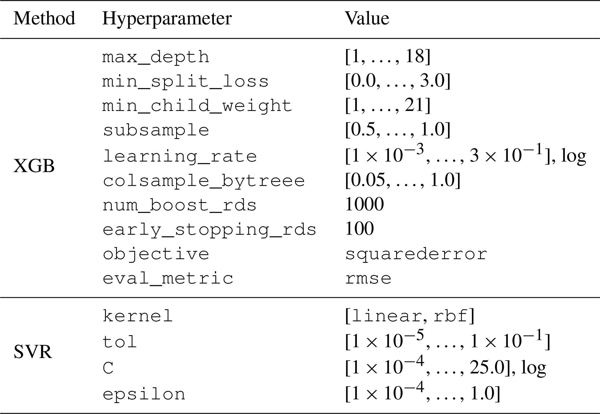
Tuning hyperparameters was done with a dedicated Python package for parameter optimisation called Optuna, v2.10.0 (Akiba et al., 2019). It provides an automated search algorithm for optimal hyperparameters. For the parameter sampling, the Tree-structured Parzen Estimator algorithm was applied (optuna.samplers.TPESampler), which is flexible and tends to converge into global minima efficiently. For each tuning study, 300 trial samplings were carried out. The investigated hyperparameter space for the XGB and SVR methods are shown in Table 1.
Table 1Hyperparameter space investigated for the machine learning algorithms XGBoosting regressor (XGB) and Support Vector Regressor (SVR), as recommended in the documentations (Chen and Guestrin, 2016; Pedregosa et al., 2011).
The comparison of the surrogates was done by first splitting the data set into a train and test data set (randomised 75 % and 25 % of the total data set, respectively). The surrogates were then trained using the train data set. The coefficient of determination R2 between the true numerical model and the surrogate model was calculated based on the unseen or test data set. The surrogate approach with the highest R2 was chosen for the toolkit. Additionally, the root mean squared error (RMSE) was calculated. If this value was too high for all approaches, LUT was used as a fallback solution, so that the user can only choose between the simulations actually performed.
2.3 One-Way Hydromechanical Coupling
The efficiency of surrogates compared to numerical models allows for loose coupling of multiple model components. In the toolkit, a one-way hydromechanical coupling was implemented using data from both contaminant transport and geomechanical models. Changes in fracture properties due to rock deformation, i.e., shear and normal displacements, can influence hydraulic properties and the resulting contaminant transport. To take this into account when quantifying the risk of aquifer contamination, changes in fracture opening are calculated from the normal displacements at each fracture section (Otto et al., 2022).
A simplified, schematic representation of the subsurface in Máza-Váralja can be seen in Fig. 2a. The model area is crossed by two regional faults that determine the groundwater discharge. Figure 2b shows the steps carried out in the hydromechanical coupling. (1) The permeability of the evolved fault sections due to normal displacement was calculated using the cubic law (Bear, 1988). (2) The effective permeability of each fault was determined analogously to a serial circuit using the harmonic mean. Then, the effective permeability was calculated analogously to a parallel circuit using the arithmetic mean of both faults. (3) This increased fault permeability was then plugged into the hydrogeological model to model contaminant transport.
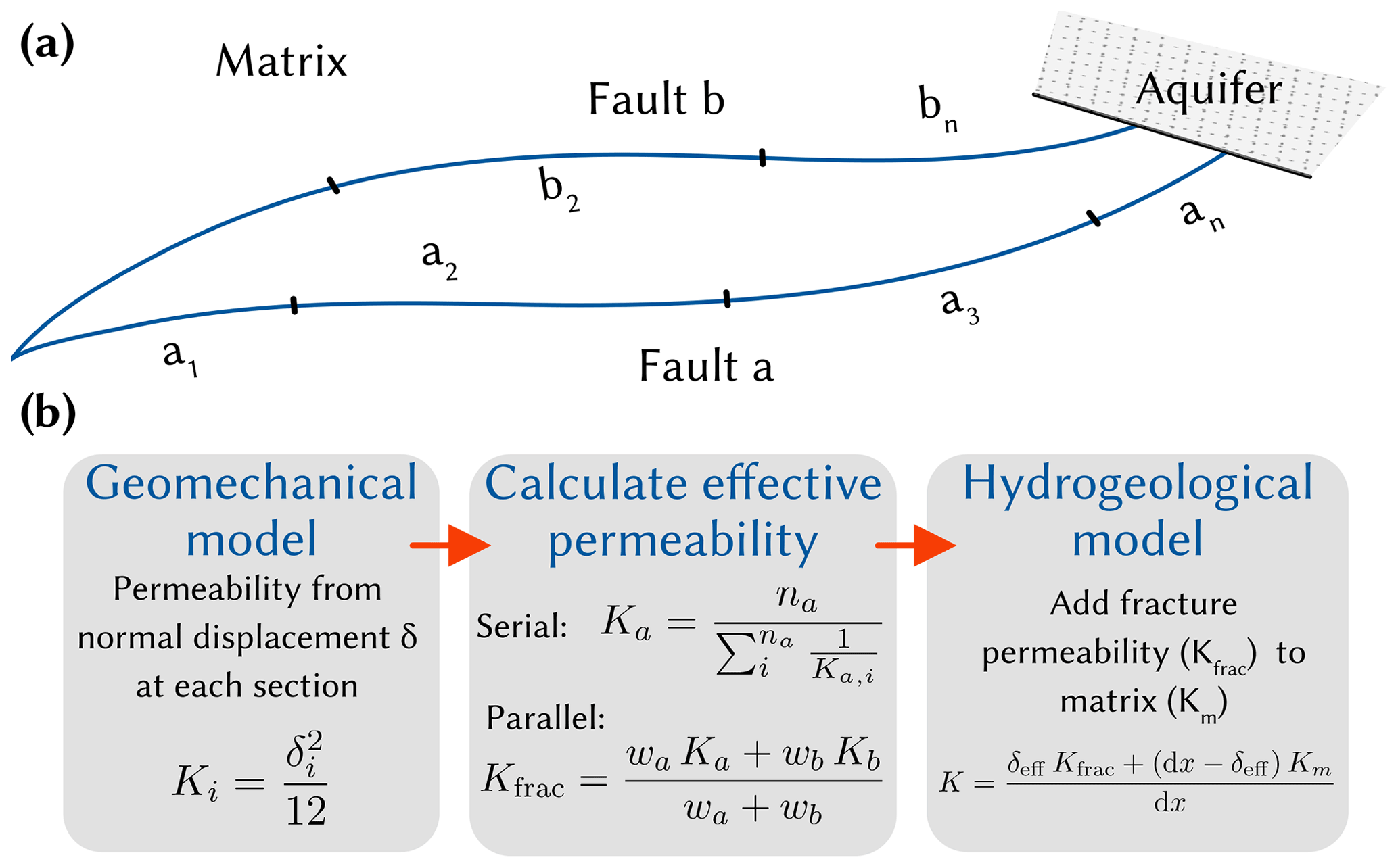
Figure 2(a) Simplified subsurface schematic of the Máza-Váralja site showing the two main regional faults which determine the discharge of the model. In the geomechanical model, subsections of each fault are monitored individually with respect to shear and normal displacements. (b) Flow chart of the implemented hydromechanical coupling, which takes changes in fracture apertures into account and updates the permeability of the hydrogeological/contaminant transport model. K is the permeability, δ is the normal displacement or aperture, n is the amount of individual sections, wx are weights based on flow cross-section.
2.4 Toolkit Application
The frontend of the toolkit was created using Streamlit, v1.9.0, a Python package for web-based dashboards (Streamlit, 2022). Each data set is represented by its own runner, which manages the user inputs (widgets), the statistical representation of the individual output parameters and the callback/update functions. These are triggered each time a widget input is changed. The initial steps for each record are as follows (performed by the runner):
-
Define input and output parameters; determine their ranges; define surrogate type.
-
If surrogate is look-up table based, then load the original data, else load the previously trained ML estimator.
-
Create an additional runtime data set. This consists of 1024 samples and is derived by uniform sampling of the input parameter ranges using Sobol's quasi Monte Carlo (QMC) sampling algorithm implemented in Scipy (Virtanen et al., 2020).
-
Calculate outputs using the surrogate and statistics of the results.
The custom runtime data set is updated each time the parameter ranges are changed. To speed up the callback functions, all data except the runtime data set is cached using Streamlit's cache function (Streamlit, 2022). This saves time in use, as the numerical model data and/or surrogate parameters would have to be loaded from disk each time.
3.1 Data Analysis
In the following, the Kardia contaminant transport dataset is analysed and processed with regard to the surrogate development. Parameter units are omitted intentionally here, as some data are transformed during this step and would have no meaningful physical unit. The main objective is to evaluate the values and parameter dependencies rather than the physical quantities, as the surrogate in the toolkit is purely data-driven.
Three input parameters were varied in the scenario analysis: the overburden hydraulic conductivity as well as the longitudinal dispersivity and the retardation coefficient of the contaminant in the overburden. It was assumed that hydraulic conductivity may increase as a result of the excavation, so values up to an order of magnitude above the predetermined baseline were investigated. The parameter was therefore converted into a simple factor of the baseline hydraulic conductivity with values from 1–10 (Xkf). The longitudinal dispersivity was varied from 10−2 to 10 m. Since this parameter spans several orders of magnitude, the logarithm was used instead (log alpha) so that each value is equally represented in the data set. The retardation coefficient (R) ranges from 1–9, and was not transformed. The scenario analysis was performed with 100 parameter sets determined by Latin Hyper Cube Sampling to achieve pseudo-random coverage of the predefined parameter ranges. Note that log alpha was drawn from a log-uniform distribution, and Xkf and R were drawn from a uniform distribution.
One model output that is shown here exemplary was the maximum concentration of the contaminant in the nearby aquifer at the defined times 10, 30, and 50 years after the abandonment and flooding of the underground construction. These discrete times steps can also be seen as an input feature of the model output to be varied in the toolkit. Simulation time was therefore treated as a categorical input parameter of the surrogate and encoded as integers (time, resulting in a total sample size of 300 (100 samples per time step). The source contaminant concentration was normalised to 1.0 g L−1, and then the logarithm was used for the model output predictions (log cmax).
Figure 3 shows the data distribution of each transformed input parameter against the logarithm of the maximum contaminant concentration in the nearby aquifer. The magnitude of the output values varies between −17.3 and −9.3 and the median is −14.7, so the output data is slightly skewed towards the lower bound. Visually, the hydraulic conductivity (Xkf) shows no correlation with contaminant transport. The dispersion parameter only has a noteworthy impact for values above 0. A clear negative and positive correlation can be seen for the retardation coefficient and the simulation time, respectively (Fig. 3c and d). This is to be expected because a higher retardation coefficient means that the contaminant is sorbed along the flow path and less contaminants will reach the aquifer. In contrast, a longer transport time leads to more contaminants entering the aquifer. It can also be seen that the model output variance increases with each time step, while the median value increases almost linearly. This indicates a non-linear effect together with the dispersion coefficient, which is responsible for an increasing plume size with transport time.
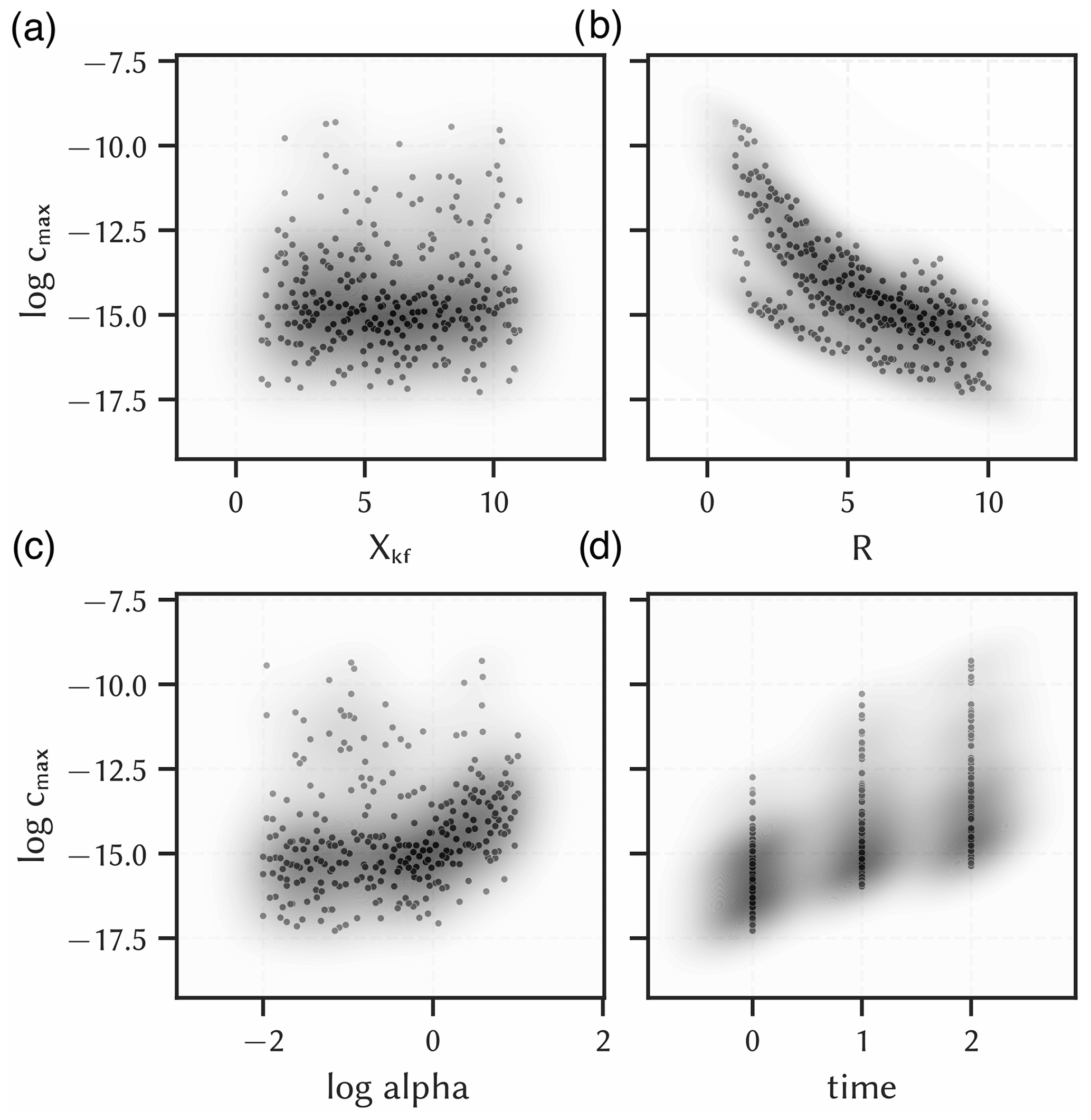
Figure 3Data distribution of all input parameters of the contaminant transport model of the Kardia site against the output maximum contaminant concentration in the aquifer (log cmax) with kernel density estimations of the points (shades). (a) hydraulic conductivity factor (Xkf), (b) logarithm of the longitudinal dispersivity (log alpha), (c) retardation coefficient (R), (d) simulation time (time). Units were left out deliberately, as some data are scaled/encoded and actual values could make no sense.
The parameter correlations were quantified with Pearson's correlation coefficients and are shown in a heatmap for all parameter couples (Fig. 4). The previously determined correlations for R and time with the model output can be confirmed here, which have correlation coefficients of about −0.7 and 0.6, respectively. For log alpha, the coefficient is only 0.19 and thus is slightly positively correlated, whereas Xkf is practically not correlated (0.07). The low correlations of the input parameters to each other are due to the stratified sampling procedure. Since the coefficient only quantifies linear correlations, but non-linear correlations can be significant, all input parameters were included in the surrogate modelling.
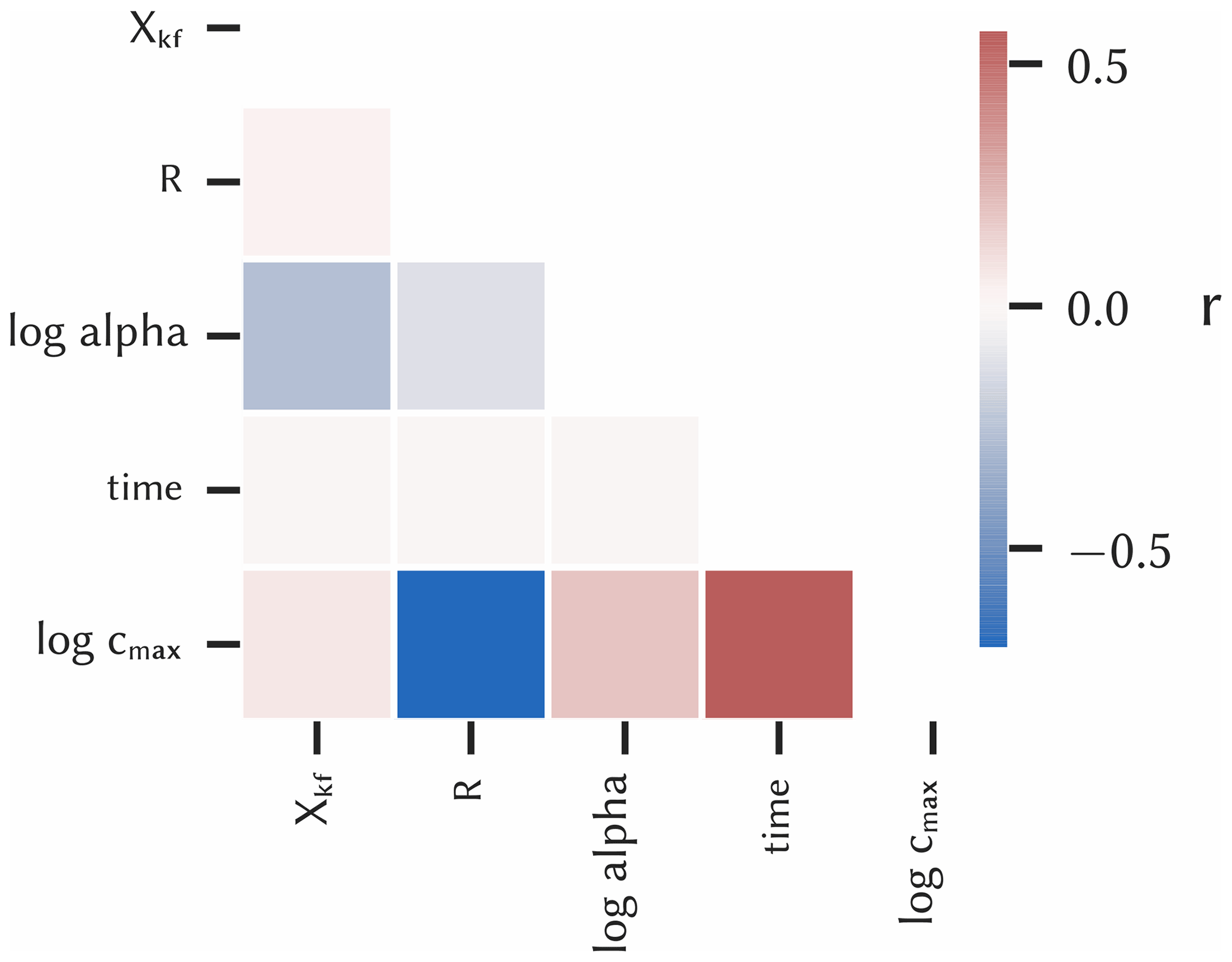
Figure 4Heatmap for the input parameters and the maximum contaminant concentration in the aquifer (log cmax) presenting Pearson's correlation coefficient r of each parameter pair.
3.2 Surrogate Selection
The pre-chosen surrogate approaches were each evaluated with two randomly splits of the data set, which are called test and train, or seen and unseen data set, respectively. The resulting true versus predicted values, i.e., the numerical and surrogate model results, and the respective errors are shown in Figs. 5 and 6.
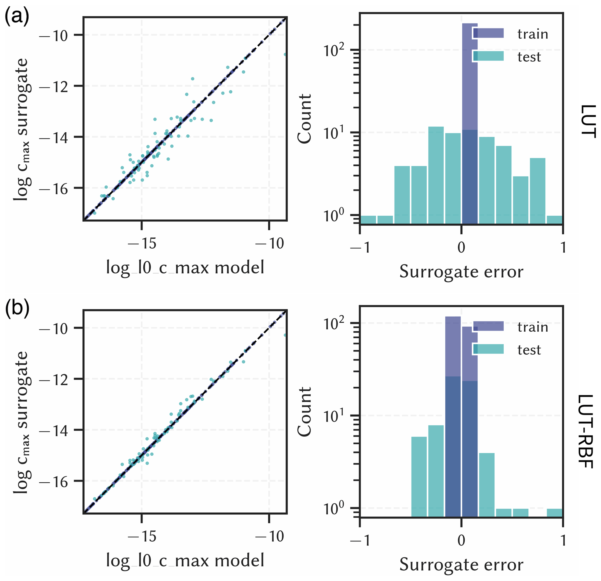
Figure 5Surrogate results for the output maximum contaminant concentration in the aquifer (log cmax) compared to numerical model results (left) and corresponding errors (right). (a) Nearest look-up table approach (LUT), (b) look-up table with radial basis function interpolation (LUT-RBF). Units are left out deliberately.

Figure 6Surrogate results for the output maximum contaminant concentration in the aquifer (log cmax) compared to numerical model results (left) and corresponding errors (right). (a) Support Vector Regression (SVR), (b) XGBoosting Regressor (XGB). Units are left out deliberately.
The look-up table methods (LUT and LUT-RBF) performed less well than the ML methods. LUT has errors ranging from −1.02 to 1.05 with a standard deviation of 0.48, and LUT-RBF has errors ranging from −0.49 to 0.96 with a standard deviation of 0.29. As this is in logarithmic scale, predictive errors of up to one order of magnitude compared to the modelled results are expected, which can be of significance in risk management. These poor results can be attributed to the relatively small sample size of the underlying scenario analysis. The precision of these look-up table based approaches can be increased by using more samples in the scenario analysis. However, this is not always possible if the underlying numerical models are complex and have a long runtime.
The machine learning algorithms (XGB and SVR), on the other hand, were better able to capture the non-linear parameter correlations and reproduce the data with lower errors. Although the error ranges are similar – −0.62 to 0.47 and −0.82 to 0.93 for SVR and XGB, respectively – the standard deviations are only 0.17 and 0.24, respectively. This suggests that there are some outliers in the predictions that are particularly erroneous, but overall the errors are normally distributed and close to zero.
The corresponding R2 values for each surrogate on the train and test data set are shown in Fig. 7. The R2 values are, as expected from the previous findings, highest for the SVR method, although the XGB method performs similarly well (both are above 0.98). Apart from fit, there seems to be no clear indication of whether one algorithm is better than another in terms of simplicity and efficiency. All surrogates worked with similar efficiency, which was ultimately not noticeable from the toolkit users' point of view. The ML methods require more configuration and parametrisation, but with special tuning packages like Optuna this can be automated to a certain extent (Akiba et al., 2019). Therefore, SVR was chosen for this dataset in the toolkit as it performed best with regard to R2 overall.
It is recommended to test different surrogate types as each dataset is unique. While XGB worked well for all investigated data sets (Kardia and Máza-Váralja), it was not always the best solution, as was the case for the here presented evaluation. In future studies, deep learning algorithms such as deep neural networks could be considered as they have a remarkable ability to adapt to non-linear, multi-parameter problems. Although their configuration is even more tedious than that of the ML methods proposed here, new tools to reduce the effort are expected in the near future. This could reduce the surrogate errors for very complex data sets.
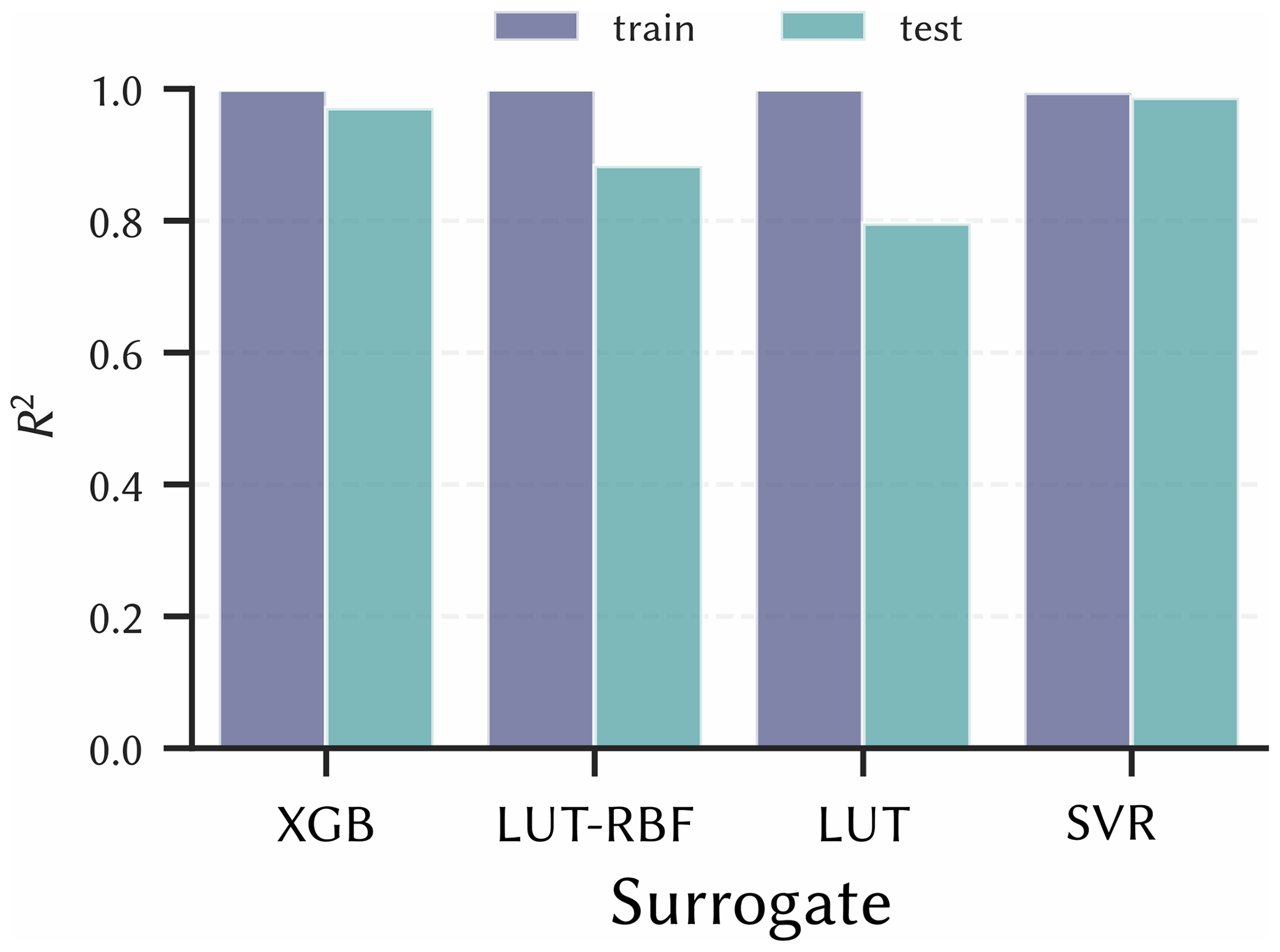
Figure 7Comparison of four different surrogate strategies using the coefficient of determination for the maximum contaminant concentration in the aquifer. All strategies do well on the train set. But, SVR has the best fit for the test set, thus it was implemented in the toolkit application.
3.3 Toolkit Application
Figure 8 showcases the contaminant transport predictions using the selected SVR surrogate in the web based dashboard. Two main areas are presented to the user: the input parameter section on the left side, and the main output section in the centre. The application is interactive so that the user can choose, which parameters or, if applicable, parameter ranges to choose from. The probabilistic hazard predictions (histograms) – in this case the maximum contaminant concentration in the nearby aquifer – will then be updated based on the chosen parameter set. Behind the scenes, a new data set will be produced, and the surrogate is used to make rapid calculations within seconds, which would take hours to days, if the original numerical model would be used.

Figure 8Prediction dashboard with interactive input parameters for the contaminant transport model of Kardia using the SVR surrogate. Different input parameter selections were used: (a) , , , and time=50. (b) , , , and time=50. A higher retardation coefficient range significantly reduces the expected contaminant concentration in the aquifer.
In Fig. 8, two different input parameter sets, and the corresponding histograms are shown. All parameters except the retardation coefficient were kept the same to highlight its specific effect on contaminant transport. The top section (Fig. 8a) presents the range of , and the lower section (Fig. 8b) presents a higher range of . While the first case is representative for a near conservative transport, the latter is a case of significant sorption along the flow path. Correspondingly, the median of the concentration probability for the conservative case is around 10−10 g L−1, and around 10−15 g L−1 for the retarded case; a difference of around five orders of magnitude.
The shown concentration values are normalised to a source concentration of 1 g L−1. In the toolkit, the source concentration and the threshold contaminant concentration are modifiable. The former multiplies the concentration data with a factor to have the actually expected source concentration. The latter adds a vertical line in the histogram plot to help visualise if a specific threshold is exceeded for the given input. These options can be used if the model should be used for a specific contaminant.
The quantification of hazards in the course of subsurface utilisation projects is essential for risk management and mitigation of environmental problems as well as for human safety. This is usually done with numerical models, as they can resolve the effects of processes in the subsurface in detail, but they have the disadvantage of being computationally intensive. For planning and managing a project, it is practically not feasible to run these models on demand. In this study, a newly developed toolkit was presented for quantifying hazards that instead uses fast, data-driven surrogate models. This allows flexible, on-demand calculations of hazard probabilities in light of updated knowledge of model input parameters.
The approach was applied to the two study areas Kardia, Greece and Máza-Váralja, Hungary as part of a risk assessment for in-situ coal conversion. The scenario analyses of the geomechanical and contaminant transport processes of the individual sites form the data basis for this study, whereby the Kardia transport model was examined in more detail here as an example. In a first step, the data were analysed and transformed with regard to parameter dependencies as well as numerical and categorical value types, which is necessary to enable surrogate modelling. Based on the data characteristics such as linear and non-linear parameter dependencies as well as experience, four surrogate algorithms were pre-selected for further comparison; two were look-up table based and two were machine learning algorithms. They were each evaluated on the basis of simplicity, goodness of fit and efficiency, with the greatest emphasis on goodness of fit, i.e., the ability to reproduce the results of the numerical model using only the input parameters.
The surrogates based on look-up tables did not perform as well, which was due to the relatively small sample size. However, due to the high complexity of the numerical models and the long simulation times, it is often not possible to create more samples. This is where machine learning algorithms come into their own, as they are able to derive complex parameter dependencies even with a limited amount of input data. They were able to reproduce previously unseen scenarios with high accuracy (R2>0.98). This made it possible to integrate quasi-immediate hazard calculations into a web-based dashboard to predict their probabilities using user-selected input parameter ranges with little accuracy trade-off.
The transparency of the assessment basis should generally increase the acceptance of geoengineering projects, which is seen as one of the crucial aspects for the further development and dissemination of geological subsurface utilisation. Furthermore, the flexibility of this approach to couple complex subsurface processes and adapt to new incoming data in terms of parameter uncertainties during a project phase can significantly increase the predictive value of hazard quantification. In principle, this newly developed tool can be used as a template for similar hazard quantification efforts, such as radioactive waste disposal, deep geothermal energy, and material energy storage.
Please contact the corresponding author for information on data and code availability.
MT, SvS, CO, and TK designed the research; MT performed the research; MT, CO, and TK analysed the data; and all authors wrote the paper.
The contact author has declared that none of the authors has any competing interests.
Publisher's note: Copernicus Publications remains neutral with regard to jurisdictional claims in published maps and institutional affiliations.
This article is part of the special issue “European Geosciences Union General Assembly 2022, EGU Division Energy, Resources & Environment (ERE)”. It is a result of the EGU General Assembly 2022, Vienna, Austria, 23–27 May 2022.
The authors appreciate the constructive comments from the topical editor and the anonymous reviewers.
This publication is part of the ODYSSEUS project that has received funding from the Research Fund for Coal and Steel (grant no. 847333).
This publication has been supported by the funding Deutsche Forschungsgemeinschaft (DFG, German Research Foundation; Open Access Publikationskosten (grant no. 491075472)).
The article processing charges for this open-access publication were covered by the Helmholtz Centre Potsdam – GFZ German Research Centre for Geosciences.
This paper was edited by Viktor J. Bruckman and reviewed by two anonymous referees.
Akiba, T., Sano, S., Yanase, T., Ohta, T., and Koyama, M.: Optuna: A next-Generation Hyperparameter Optimization Framework, in: Proceedings of the 25rd ACM SIGKDD International Conference on Knowledge Discovery and Data Mining, https://doi.org/10.1145/3292500.3330701, 2019. a, b
Bear, J.: Dynamics of Fluids in Porous Media, Dover Books on Physics and Chemistry, Dover, New York, 1988. a
Chen, T. and Guestrin, C.: XGBoost: A Scalable Tree Boosting System, in: Proceedings of the 22nd ACM SIGKDD International Conference on Knowledge Discovery and Data Mining, KDD '16, ACM, New York, NY, USA, 785–794, https://doi.org/10.1145/2939672.2939785, 2016. a, b
Géron, A.: Hands-on Machine Learning with Scikit-Learn and TensorFlow: Concepts, Tools, and Techniques to Build Intelligent Systems, O'Reilly Media, ISBN 9781491962268, 2017. a
Goldsim Technology Group: GoldSim User's Guide (Version 14.0), Tech. rep., 2021. a
Hedayatzadeh, M., Sarhosis, V., Gorka, T., Hámor-Vidó, M., and Kalmár, I.: Ground Subsidence and Fault Reactivation during In-Situ Coal Conversion Assessed by Numerical Simulation, Adv. Geosci., accepted, 2022. a, b
Kempka, T., Nakaten, N., Gemeni, V., Gorka, T., Hámor-Vidó, M., Kalmár, I., Kapsampeli, A., Kapusta, K., Koukouzas, N., Krassakis, P., Louloudis, G., Mehlhose, F., Otto, C., Parson, S., Peters, S., Pyrgaki, K., Roumpos, C., Sarhosis, V., and Wiatowski, M.: ODYSSEUS – Coal-to-liquids Supply Chain Integration in View of Operational, Economic and Environmental Risk Assessments under Unfavourable Geological Settings, in: Proceedings of the 38th Annual Virtual International Pittsburgh Coal Conference, 38th Annual International Pittsburgh Coal Conference 2021: Clean Coal-based Energy/Fuels and the Environment, PCC 2021, 2021, 2, pp. 858–866, 2021. a
Krassakis, P., Pyrgaki, K., Gemeni, V., Roumpos, C., Louloudis, G., and Koukouzas, N.: GIS-Based Subsurface Analysis and 3D Geological Modeling as a Tool for Combined Conventional Mining and In-Situ Coal Conversion: The Case of Kardia Lignite Mine, Western Greece, Mining, 2, 297–314, https://doi.org/10.3390/mining2020016, 2022. a
Oladyshkin, S.: Efficient Modeling of Environmental Systems in the Face of Complexity and Uncertainty, https://doi.org/10.18419/OPUS-615, 2014. a
Otto, C., Steding, S., Tranter, M., Gorka, T., Hámor-Vidó, M., Basa, W., Kapusta, K., Kalmár, I., and Kempka, T.: Numerical Analysis of Potential Contaminant Migration from Abandoned In Situ Coal Conversion Reactors, Adv. Geosci., 58, 55–66, https://doi.org/10.5194/adgeo-58-55-2022, 2022. a, b, c
Pedregosa, F., Varoquaux, G., Gramfort, A., Michel, V., Thirion, B., Grisel, O., Blondel, M., Prettenhofer, P., Weiss, R., Dubourg, V., Vanderplas, J., Passos, A., Cournapeau, D., Brucher, M., Perrot, M., and Duchesnay, E.: Scikit-Learn: Machine Learning in Python, J. Mach. Learn. Res., 12, 2825–2830, 2011. a, b, c, d
Streamlit: V1.9.0, https://streamlit.io/ (last access: 20 April 2022), 2022. a, b
Virtanen, P., Gommers, R., Oliphant, T. E., Haberland, M., Reddy, T., Cournapeau, D., Burovski, E., Peterson, P., Weckesser, W., Bright, J., van der Walt, S. J., Brett, M., Wilson, J., Millman, K. J., Mayorov, N., Nelson, A. R. J., Jones, E., Kern, R., Larson, E., Carey, C. J., Polat, İ., Feng, Y., Moore, E. W., VanderPlas, J., Laxalde, D., Perktold, J., Cimrman, R., Henriksen, I., Quintero, E. A., Harris, C. R., Archibald, A. M., Ribeiro, A. H., Pedregosa, F., van Mulbregt, P., and SciPy 1.0 Contributors: SciPy 1.0: Fundamental Algorithms for Scientific Computing in Python, Nat. Meth., 17, 261–272, https://doi.org/10.1038/s41592-019-0686-2, 2020. a, b