Numerical Analysis of Potential Contaminant Migration from Abandoned In Situ Coal Conversion Reactors

In the context of a potential utilisation of coal resources located in the Mecsek mountain area in Southern Hungary, an assessment of groundwater pollution resulting from a potential water-borne contaminant pool remaining in in situ coal conversion reactors after site abandonment has been undertaken in the scope of the present study. The respective contaminants may be of organic and inorganic nature. A sensitivity analysis was carried out by means of numerical simulations of fluid flow as well as contaminant and heat transport including retardation to assess spatial contaminant migration. Hereby, the main uncertainties, e.g., changes in hydraulic gradient and hydraulic contributions of the complex regional and local fault systems in the study area, were assessed in a deterministic way to identify the relevant parameters. Overall 512 simulations of potential groundwater contamination scenarios within a time horizon exceeding the local post-operational monitoring period were performed, based on maximum contaminant concentrations, cumulative mass balances as well as migration distances of the contaminant plume. The simulation results show that regional faults represent the main contaminant migration pathway, and that contamination is unlikely assuming the given reference model parametrisation. However, contamination within a simulation time of 50 years is possible for specific geological conditions, e.g., if the hydraulic conductivity of the regional faults exceeds a maximum value of 1 × 10⁻⁵ m s⁻¹. Further, the parameter data analysis shows that freshwater aquifer contamination is highly non-linear and has a bimodal distribution. The bivariate correlation coefficient heatmap shows slightly positive correlations for the pressure difference, the fault permeability and the simulation time, as well as a negative correlation for the retardation coefficient. The results of this sensitivity analysis have been integrated into a specific toolkit for risk assessment for that purpose.

1 Introduction

The present study aims at the implementation of a sensitivity analysis by means of coupled numerical process modelling to assess potential environmental impacts at a prospective in situ coal conversion site in Máza-Váralja (Hungary). In this context, the post-operational monitoring period is specifically investigated in view of potential groundwater aquifer contamination in the long term, considering various hydrogeological uncertainties of the study area. The post-burn process operation is critical for reducing in situ coal conversion impacts on groundwater quality. It implies steam injection into and production from the reactors for cooling and venting, and thus removing effluents. Thereby, postburn pyrolysis is minimsed (Sury et al., 2004), which is assumed as initial state in the models in the present study. Hereby, soluble organic contaminants, such as benzene or phenols, may migrate beyond the in situ coal conversion reactors (Beath et al., 2004).

In the scope of the EU-RFCS project ODYSSEUS, a toolkit was developed from scratch to assess the probability of environmental hazards and risks associated with in situ coal conversion. The publication of Tranter et al. (2022) (this issue) describes in detail the theoretical background of this toolkit, as well as its handling and application, targeted for operators, stakeholders and regulators (e.g., mining authorities and environmental agencies). In order to be able to quantify environmental hazards and forecast potential outcomes, it is crucial to identify the process-related environmental impacts (e.g., groundwater contamination, surface subsidence, induced seismicity, etc.) first. In the scope of that overarching study, different numerical models were developed to account for solute transport as well as geomechanics to determine the likelihood and severity of different potential hazards. These complex numerical models, however, are computationally expensive as they show a high uncertainty of input parameters (occasionally of several orders of magnitude), and therefore require a large number of model realisations.

The results presented in this manuscript are an essential part of the toolkit and serve as data basis for the probability assessment on the environmental hazard of groundwater contamination considering a high uncertainty of the input parameters. Further, for the Máza-Váralja site, a hydro-mechanical coupling was implemented by numerically determining the hydraulic aperture change of the geological faults. Here, the effective fracture permeability is determined based on the normal displacements of the faults calculated in the geomechanical models (detailed results on the geomechanical models are presented by Hedayatzadeh et al., 2022 in the same issue) and then updated in the contaminant transport model by means of a sequential coupling.

1.1 In situ Coal Conversion

The concept of in situ coal conversion is based on borehole mining, whereby the target coal deposits are developed by directional drilling. The in situ coal conversion process starts with the ignition of the coal at the beginning of the gasification channel, which is then converted into a high-calorific synthesis gas by sub-stoichiometric combustion, using an oxidiser based on oxygen-enriched air and/or steam (Burton et al., 2006).

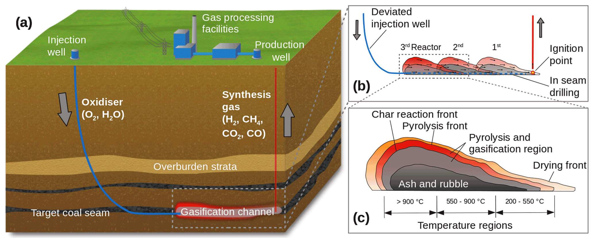
Figure 1 (a) Schematic view (not to scale) of the principle of in situ coal conversion based on the linear CRIP (Controlled Retracting Injection Point) method modified after Kempka et al. (2011). (b) Near-field view of the in situ coal conversion channel with directional drilling design and stepwise reactor excavation. (c) Regions of specific temperatures and chemical reactions in and around the in situ coal conversion reactor.

The coal conversion reactor is composed of three regions, comprising drying, coal pyrolysis and solid char gasification (Thorsness and Rozsa, 1978). The high-calorific synthesis gas constituents are mainly a mixture of H₂, CO, CO₂ and CH₄ in addition to N₂ and minor components such as sulfuric acids (Friedmann et al., 2009). Compositions and calorific values of the synthesis gas strongly depend on the thermodynamic conditions of the operation as well as on the composition and temperature of the oxidiser employed (European Commission et al., 2012; Otto and Kempka, 2020). The in situ coal conversion process has a zonal nature and the main gasification reactions occur both in presence of solid and gaseous phases (Fig. 1).

Along with the migration of the synthesis gas, resulting from thermal coal decomposition, through the pores and cleats of the coal matrix, various homogeneous and heterogeneous chemical reactions take place. Hereby, heterogeneous reactions occur at the phase boundaries in the gasification channel, while the homogeneous ones take place in the reactor pore space and open void.

1.2 Formation of By-Products During In situ Coal Conversion

The main challenges associated with in situ coal conversion operation are the potential pollutant migration out of the reactor and surface subsidence (Roddy and Younger, 2010). The collapse of an in situ coal conversion reactor as a result of ongoing coal consumption by the combustion process may generate potential migration fluid flow pathways in the coal and its roof rocks, so that undesired gasification by-products, such as organic (phenols, benzene, PAHs, etc.) and inorganic pollutants (ammonia, sulphates, cyanides and heavy metals, etc.) may exit the reactor in an uncontrolled manner (Humenick and Mattox, 1978; Kapusta and Stańczyk, 2011; Liu et al., 2007).

Leakage of oxidation agents and synthesis gases may occur if the process is operated in the vicinity of major geologic faults (Burton et al., 2006; Creedy and Garner, 2004). In addition, faults and fractures may support the migration of in situ coal conversion gases, trigger groundwater flow in unexpected directions and provide pathways for contaminant migration into shallow fresh water aquifers.

Besides, ground surface subsidence may occur due to coal extraction, and induce damage to surface infrastructure and the environment. The factors that influence the stresses developed in the overlying formation, dictating the extent of fracturing and the likelihood of subsidence include: (1) the coal seam thickness; (2) the in situ coal conversion reactor width (Shu and Bhattacharyya, 1993); (3) the depth and mechanical strength of the hanging wall (overlying geology); and (4) the presence of geologic fault systems.

In general, gasification is operated at higher temperatures and produces low-molecular-weight gases that can be efficiently produced from the in situ coal conversion reactor. In contrast, pyrolysis occurs at lower temperatures and produces high molecular-weight compounds, of which some readily condense in the reactor. Many of these are well-known groundwater contaminants and difficult to extract from the coal conversion residues left in the subsurface (Blinderman et al., 2008).

Nevertheless, in situ coal conversion has a significantly lower environmental footprint compared to conventional mining, since coal is not mechanically excavated, transported to the surface, processed and combusted or gasified in a surface plant. Also, in situ coal conversion generates significantly smaller volumes of waste products (e.g., fly ashes) as well as pollutants, and moreover induces lower dust pollution, water consumption and methane emissions into the atmosphere. Coupled with existing technologies for carbon dioxide capture and storage (CCS) or even CO₂ utilisation to produce chemical feedstock such as methanol, in situ coal conversion has the potential to recover energy from coal with a low CO₂ footprint (Roddy and Younger, 2010; Sarhosis et al., 2013; Nakaten and Kempka, 2019).

2 Material and Methods

2.1 Study Area Máza-Váralja (Hungary)

The Máza-Váralja coal deposit is located in the North-east Mecsek mountain area about 190 km SWS from Budapest (Hungary), providing an infrastructure comprising road and railway connections as well as water and energy supply. The currently active mining license extends to about 10.6 km², comprising 20 mineable coal seams of 1.4 to 3.4 m thickness and total coal resources of 438 Mt, whereof 280 Mt are mineable reserves. One third of the coal resources is located at depths up to 600 m below ground level (m b.g.l.) at an average dip angle of ≤ 30^∘, whereby two thirds of the resources are situated at depths up to 1100 m b.g.l. at dip angles of ≤ 40 to 60^∘. The complex-structured Mesozoic coal deposit consists of ash- and sulphur-rich, high-volatile coals with a methane content of 20–50 m³ per ton of coal. Three main types of fault systems (basin-margin normal-growth faults, reverse faults, late-stage thrust faults) subdivide the target area into seven coal blocks (GEOS, unpublished report, 2009; S. Klich, unpublished report, 2010; B. Fodor, unpublished data, 2012; L. Bacskó et al., unpublished report, 2010).

Conventional coal mining in the Máza-Váralja coal deposit was stopped in 2004 due to the general Hungarian energy policy as well as the low oil and gas prices at this time. The deposit has been explored for many decades by means of more than 30 boreholes and 2D and 3D seismic campaigns, providing a sound understanding of its geology and variability in coal quality. Preliminary geological data already approved by Hungarian authorities, seismo-tectonic studies on geologic fault locations and pre-feasibility studies on the development of the coal deposit have been elaborated (Püspöki et al., 2012).

2.2 Gasification By-Products Obtained From Ex situ Experiments

In the scope of a higher-level interdisciplinary study, large-scale experimental testing on Máza-Váralja bulk coal samples were undertaken to determine and quantify the in situ coal conversion by-products as well as the gasification efficiency depending on different $p/T$ conditions and oxidiser compositions.

Although the main purpose of the in situ coal conversion process is to efficiently convert coal into a high-calorific synthesis gas, the process is inextricably linked with the formation of a number of gasification by-products. Most of these are known to be hazardous to the environment, both during the production phase and after site abandonment. This is mainly due to the potential release of different organic (i.e. BTEX, PAHs, phenols) and inorganic pollutants (i.e. heavy metals). The main by-products remaining in the subsurface after site abandonment include: (1) tars – composed of volatile coal pyrolysis products condensed in the wells and pipelines; (2) coal conversion wastewater – formed as a result of synthesis gas cooling, condensation and mixing with inflowing groundwater in low-temperature zones of the reactor; (3) solid gasification residues – ash and char formed during coal conversion left in the reactor.

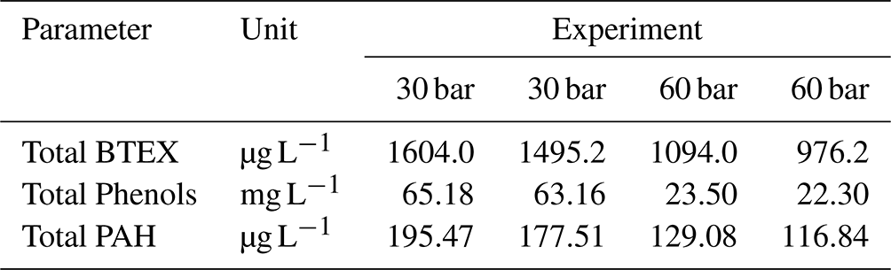
During the ex situ experiments, the gasification by-products were produced and sampled, and then analysed with regard to their chemical composition. The average total phenol concentrations of the gasification wastewater of the Máza-Váralja coal bulk samples were about 64.2 and 22.9 mg L⁻¹ at operational pressures of 30 and 60 bar, respectively.

Phenols are characterised by low-molecular weight, low sorption capacities, and especially by high aqueous solubility. Hence, their potential migration into fresh water aquifers may be supported by local and regional groundwater flow. The effect of gasification pressure on the organic composition of the wastewater is evident: an increase in gasification pressure significantly decreases the concentrations of all three groups of organic compounds (Phenols, BTEX, PAHs; Table 1), which is considered as a typical phenomenon.

Table 1 Average concentrations of organic compounds of the in situ gasification wastewater of the Máza-Váralja coal bulk samples.

With an odour and taste threshold value of 1 µg L⁻¹ for drinking water proposed by the Federal Environmental Agency of Germany, risk for human health and the environment are not given at this concentration (IHCP, 2006).

The laboratory experiments on the water-borne contaminants show the high uncertainty range of possible organic contaminant concentrations depending on, e.g., coal seam depth. In the numerical simulations carried out in the present study, a probabilistic approach is therefore applied to take this and other relevant uncertainties into account.

2.3 Fluid Flow and Transport Model

Groundwater flow and contaminant transport simulations were performed by means of the fluid flow and transport code TRANSPORT Simulation Environment (TRANSPORTSE) (Kempka, 2020; Kempka et al., 2022). It considers pressure- and density-driven fluid flow, convective and conductive heat transport, as well as advective, diffusive and dispersive chemical species transport. The aim of the simulations was to assess and quantify the contaminant migration from the target coal seams into the freshwater aquifer in the study area.

2.4 Model Geometry

The cross section investigated in the present study is derived from the mechanical model introduced by Hedayatzadeh et al. (2022) (this issue), which has been developed in the scope of the aforementioned higher-level interdisciplinary study to account for possible hydromechanical impacts of the in situ coal conversion operation, e.g., changes in geologic fault apertures due to fault reactivation. For the present flow and transport simulations, a 2D numerical model with a spatial extent of 2000 m × 1150 m has been extracted. It includes the target coal seams and their surrounding aquitards, the relevant geologic faults which may act as potential contaminant migration pathways, and the freshwater aquifer connected to these faults (Fig. 2). A uniform discretisation of 200 × 115 elements is applied, corresponding to a element size of 10 m × 10 m.

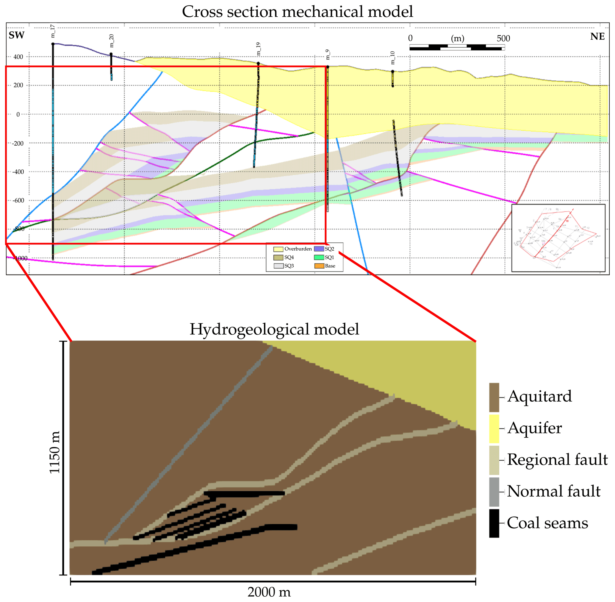
Figure 2 Geological cross section of the Máza-Váralja study area. The thermo-hydrogeological model is derived from the mechanical model from Hedayatzadeh et al. (2022). Reverse faults (pink) are neglected due to their limited hydrogeological relevance.​​​​​​​

The lithology in the study area is highly variable. Coal seams are located in different Lower Jurassic rock types (marl, sandstone, limestone), which are highly compacted, and therefore considered as aquitards (Fig. 2, brown). Hydraulic conductivity is defined by uniform values for all of the aquitard units (1 × 10⁻⁸–5 × 10⁻⁹ m s⁻¹). The freshwater aquifer (Fig. 2, yellow) belongs to the Miocene series and mainly consists of unconsolidated sand, gravelly sand and conglomerates with marl and clay marl interbeddings. Its hydraulic conductivity is in the range of 5 × 10⁻⁸ and 5 × 10⁻⁶ m s⁻¹.

Geologic fault zones are distinguished into normal, regional and reverse faults. The normal faults show the highest hydraulic conductivity (1 × 10⁻³–1 × 10⁻⁵ m s⁻¹), while the regional ones exhibit a significantly lower conductivity (1 × 10⁻⁵–1 × 10⁻⁷ m s⁻¹), and the reverse faults are hydrogeologically inactive unless mechanical normal displacements generate an aperture. Thus, the present modelling work focusses on the normal (Fig. 2, grey) and regional faults as potential fluid flow and contaminant migration pathways (Fig. 2, beige).

2.5 Initial and Boundary Conditions

The model topography was simplified introducing a constant-elevation boundary at the model top which is derived from the hydraulic head at the right model boundary.

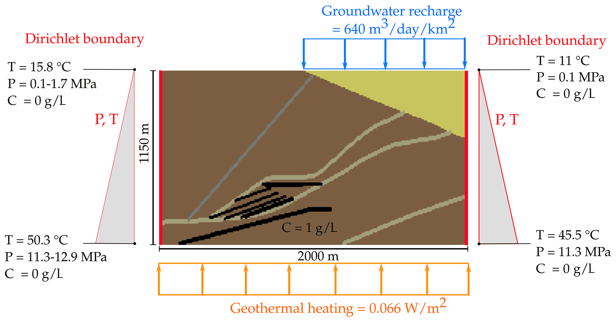
Figure 3 Initial and boundary conditions of the thermo-hydrogeological model. Differences in model topography are represented by the increased $p/T$ conditions at the left model boundary.

As mining with water management is planned in the study area, post-operational flooding will lead to relatively fast hydraulic head changes in the entire model domain. Therefore, the initial and boundary conditions were chosen based on information available on the topography. Pressure and temperature variations with depth are considered according to the hydraulic and geothermal gradients, and pre-equilibrated in the model to achieve an initial steady state for each simulation run. Dirichlet conditions are applied at the left and right model boundaries with constant temperatures, pressures and concentrations. This represents a conservative assumption to take into account expected hydraulic head changes due to water management, so that the extreme values are part of the sensitivity study. At the left boundary, the ground surface is about 160 m higher than that at the right one, which is considered by means of higher temperatures (and pressures) at the respective locations (Fig. 3).

Dirichlet boundary conditions are used to employ constant temperatures, pressures and concentrations at the right and left model boundaries. A surface temperature of 11 ^∘C is assumed, corresponding to the annual average of the Máza-Váralja region. Below the surface, a linear increase in temperature of 0.03 K m⁻¹ is assumed, resulting in a temperature of 15.8 ^∘C at the upper left model boundary (Fig. 3). Within the model, an initial hydrostatic pressure distribution is assumed, corresponding to a pressure of one atmosphere (1.01325 bar) at the top of the right model boundary and its density-dependent increase towards the model bottom. Within the aquitard at the left model boundary, the hydraulic head is uncertain, so that the applied pressures are varied between 0.1 and 1.7 MPa at this location in the context of the present uncertainty study (Fig. 3). Hereby, the higher pressure corresponds to a hydraulic head at the ground surface of the left model boundary, which is located about 160 m above the right one. In both cases, the entire model area is assumed to be fully saturated with groundwater. Contaminant concentrations at the left and right model boundaries are zero.

Initial horizontal temperature and pressure distributions are equal for all elements at the start of the simulations, except for the that at the left boundary condition, which is varied in the range of uncertainty. With regard to the aquifer, a spatial specific groundwater recharge of 640 m³ d⁻¹ km⁻² is applied at the model top (Zoltán ​​​​​​​Püspöki, unpublished report, 2009). Geothermal heat flow at the model bottom is assumed to 0.066 W m⁻² (Fig. 3). A passive tracer is used to represent the migration of any water soluble contaminant from the coal seams into the fresh water aquifer. Its concentration is normalised, i.e. a value of 1 g L⁻¹ is initially present within the in situ coal conversion reactors (Fig. 3). Any other source concentration can be considered by multiplying the results with the corresponding factor.

A threshold concentration of < 1 × 10⁻⁹ g L⁻¹ corresponds in our consideration to “no occurrence”, since a phenol threshold value of 1 µg L⁻¹ for drinking water is proposed (e.g., Federal Environmental Agency of Germany).

An average value of 5 × 10⁻⁹ m² s⁻¹ was assumed for the diffusion coefficient.

2.6 Fluid and Rock Properties

For the entire model area, the porous medium approach is applied. Hereby, the porosities of the different implemented lithological units and faults are related to their hydraulic conductivities, which have a certain bandwidth (Zoltán ​​​​​​​Püspöki, unpublished report, 2009). Table 2 shows the data used for model parametrisation.

Table 2 Porosities and hydraulic conductivities used for model realisations.

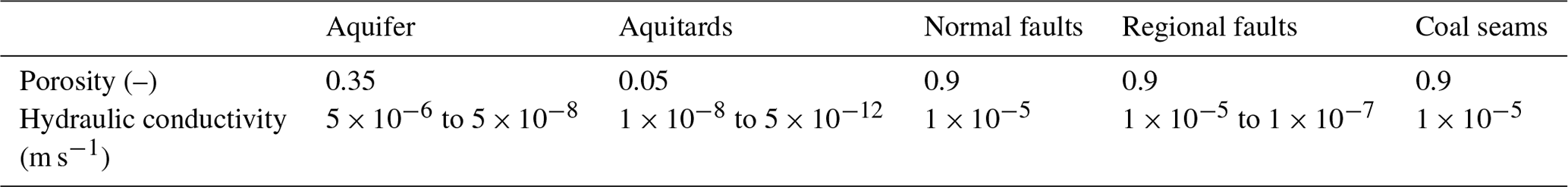
In case of the aquitards, the range of hydraulic conductivities were extended to include very low values, representing fluid flow barriers. For the normal fault, which is located left to the coal seams (Figs. 2 and 3), a minimum hydraulic conductivity is chosen.

For the coal seams, similar hydraulic conductivities as for the normal fault are applied. In the course of the sensitivity analysis, the hydraulic conductivities were varied for all other regions at constant porosities. All other rock properties are assumed to be constant and homogeneous within the modelling area. The specific heat capacity of the rocks is 850 J kg⁻¹ K⁻¹, thermal conductivity is 2 W m⁻¹ K⁻¹ and rock density is 2700 kg m⁻³ following a report by the Hungarian Geological Survey (Zoltán ​​​​​​​Püspöki, unpublished report, 2009).

Fluid properties, namely density, viscosity, thermal conductivity and heat capacity, are dynamically updated after each time step based on the local $p/T$ conditions. Thereby, interpolation functions based on the NIST database (Lemmon et al., 2021) are applied with the fluid compressibility calculated according to local pressure and density changes. Rock and fluid compressibility was initially set to 4.5 × 10⁻¹⁰ Pa⁻¹.

2.7 Hydromechanical Coupling

Changes in fault apertures due to mechanical effects, i.e., shear and normal displacements, which result from coal consumption influence the hydraulic fault properties, and thus affect potential contaminant migration along these faults.

The changes in fault permeability due to mechanical effects were assessed in a separate sensitivity study undertaken by Hedayatzadeh et al. (2022) (this issue) using a 3D mechanical model of the presented study area. The bandwidth of the calculated mechanical fault aperture changes were used as initial conditions in the present sensitivity analysis on potential aquifer contamination as follows. Mechanically-induced changes in fault apertures are calculated using the fault-specific normal displacements determined in the mechanical simulation model. Thereby, the average permeability k_avg of an element containing a fault is calculated from the documented fault permeability, k_f, and that of the surrounding rock matrix, k_m. The fault permeability k_f depends on the fault aperture a, which is calculated from the normal displacements of the respective fault section. Equation (1) is used to determine the average permeability k_avg of the respective model element, depending on its spatial dimension perpendicular to the fracture face (with Δi defined as cell width).

$$\begin{array}{}\text{(1)}& k_{\mathrm{avg}}={\displaystyle \frac{k_{\mathrm{m}}\cdot \left(\mathrm{\Delta }i-a\right)+k_{\mathrm{f}}\cdot a}{\mathrm{\Delta }i}},\text{with}{k}_{\mathrm{f}}={\displaystyle \frac{a^{\mathrm{2}}}{\mathrm{12}}}\end{array}$$

Figure 4 shows the impact of fault aperture on the fault element permeability depending on the initial rock matrix permeability. For that purpose, aperture values are derived from the mechanical simulations in the present uncertainty assessment, based on a one-way coupling between the mechanical and contaminant transport models.

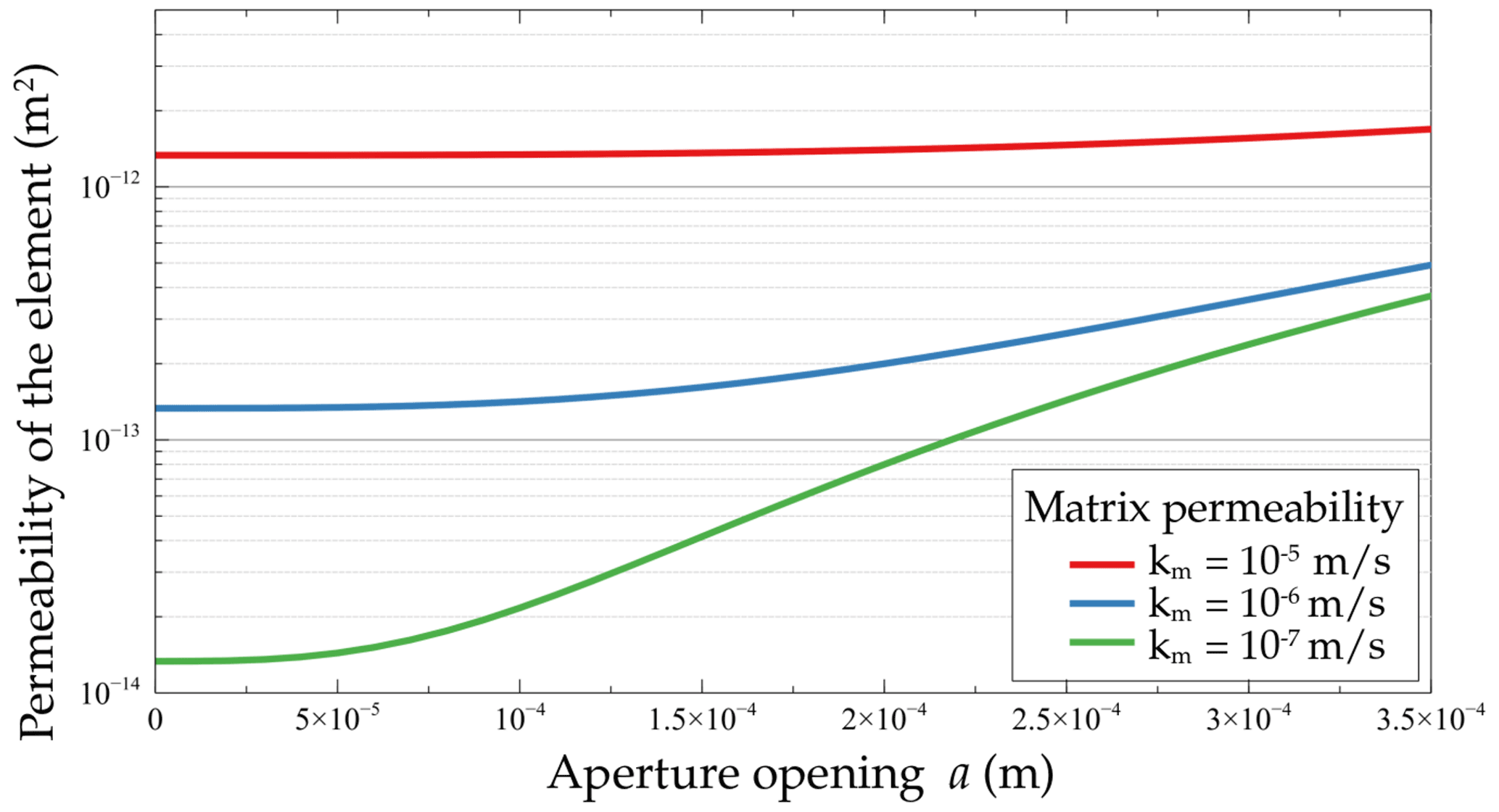
Figure 4 Permeability changes as function of the fault aperture bandwidth calculated by the mechanical model for rock matrix permeabilities representative for the Máza-Váralja study area.

3 Results and Discussion

A sensitivity analysis of a potential aquifer contamination in the Máza-Váralja study area was investigated by the variation of different input parameters within the known limits of uncertainty. For that purpose, seven input parameters were taken into account in the numerical thermo-hydrogeological simulation model: (1) the mechanically-induced changes in fault apertures, (2) the topographically-driven hydraulic head differences between the left and right model boundaries, (3) the longitudinal dispersion length, (4) the hydraulic conductivity of the fresh water aquifer, (5) the hydraulic conductivity of the aquitard, (6) the hydraulic conductivity of the regional faults, and (7) the retardation coefficient. Table 3 shows the upper and lower limits of each of these model parameters. The input parameter space was derived using Sobol's Quasi-Monte Carlo (QMC) method with 512 samples.

Table 3 Parameter variations applied in the uncertainty analysis. Seven input parameters were varied in 512 simulations based on Sobol's Quasi-Monte-Carlo (QMC) sampling method.

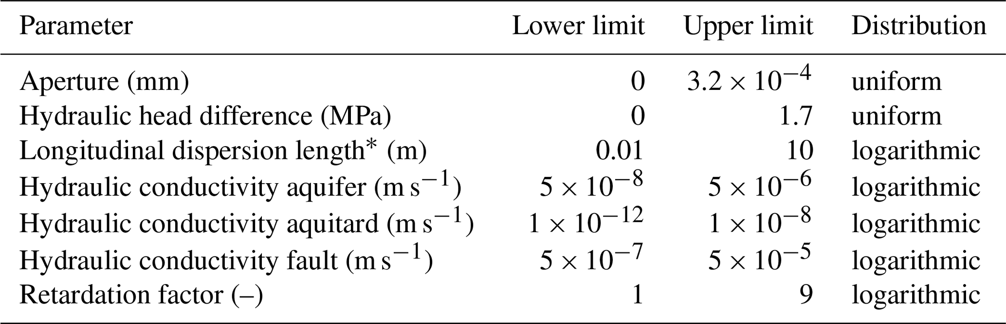
^∗ Constant longitudinal-to-transversal dispersion length ratio of 10 : 1 is applied.

3.1 Sensitivity Analysis

A sensitivity analysis was conducted to assess the impact of the different model parameters on the contaminant migration and its distribution within the hydrogeological system. Six simulation results from the 512 model runs on the spatial distribution of the contaminant plume are presented and discussed exemplarily in the following.

For the reference case, average parameter values were used. However, since not all contaminants exhibit retardation effects, and using an average retardation factor would conceal the effect of most other parameter changes, a minimum value was chosen as a conservative approach. Based on the reference case, different scenarios were tested by consecutively changing each parameter according to the minimum and maximum values given in Table 2 and comparing the simulation results with the reference case.

Furthermore, a worst-case scenario was generated, where all hydraulic conductivities and the topographically-driven hydraulic head difference were set to their maximum values while neglecting retardation, so that a maximum contaminant migration distance is achieved.

In all cases, a time period of 50 years was simulated to cover any legally relevant post-operational monitoring period, which commonly do not exceed 30 years.

Figure 5 shows the spatial concentration distributions for the reference case after simulation times of 30 and 50 years. To ensure that even small legally-allowable concentration threshold values can be considered in the result interpretation, tracer concentrations of ≥ 1 × 10⁻⁸ g L⁻¹ are used in the present assessment. The simulation results show that the regional fault located in the model middle acts as a main contaminant migration pathway. However, the fluid flow velocity is relatively low, so that about half the distance to the aquifer is crossed after a simulation time of 50 years. Accordingly, even contaminants without any retardation are not expected to reach the freshwater aquifer within this time if average pressure gradients between the lateral model boundaries and average hydraulic conductivities are assumed. Nevertheless, contaminant concentrations within the regional faults are relatively high, and hence contaminant arrival in the aquifer is conceivable at a later time.

Figure 5 Spatial concentration of contaminant simulated for the reference case after a simulation time of 30 years (a) and 50 years (b).

Changes in the hydraulic conductivity of the aquitard mainly affect the size of the contaminant plume but not its migration distance towards the aquifer. As there is no significant difference in the low hydraulic conductivity case to the reference one, diffusion is the dominant transport mechanism in this case as well. For high hydraulic conductivities, advection dominates the contaminant transport and the size of the contaminant plume increases. Nevertheless, the geologic faults remain the main migration pathways for the contaminant plume. Thereby, the spatial spread of the contaminants causes an increase in the mass transported along the upper regional fault. Also the lower regional fault is reached by the contaminants. However, the transport along the middle regional fault is decisive for the contamination of the freshwater aquifer. As long as the contaminants do not reach the normal fault at the left, the hydraulic conductivity of the aquitard has only a minor impact.

In contrast, the hydraulic conductivity of the regional faults has a major impact on the contaminant migration into the fresh water aquifer. Figure 6 shows that in case of minimum hydraulic conductivities of the regional faults, contaminant transport is negligible, whereas according maximum values cause the previously defined threshold limit of 1 × 10⁻⁸ g L⁻¹ for phenols to be exceeded. After 50 years, a contaminant plume with concentrations of up to 0.12 g L⁻¹ (12 % of the source concentration) is found within the aquifer (Fig. 6, bottom).

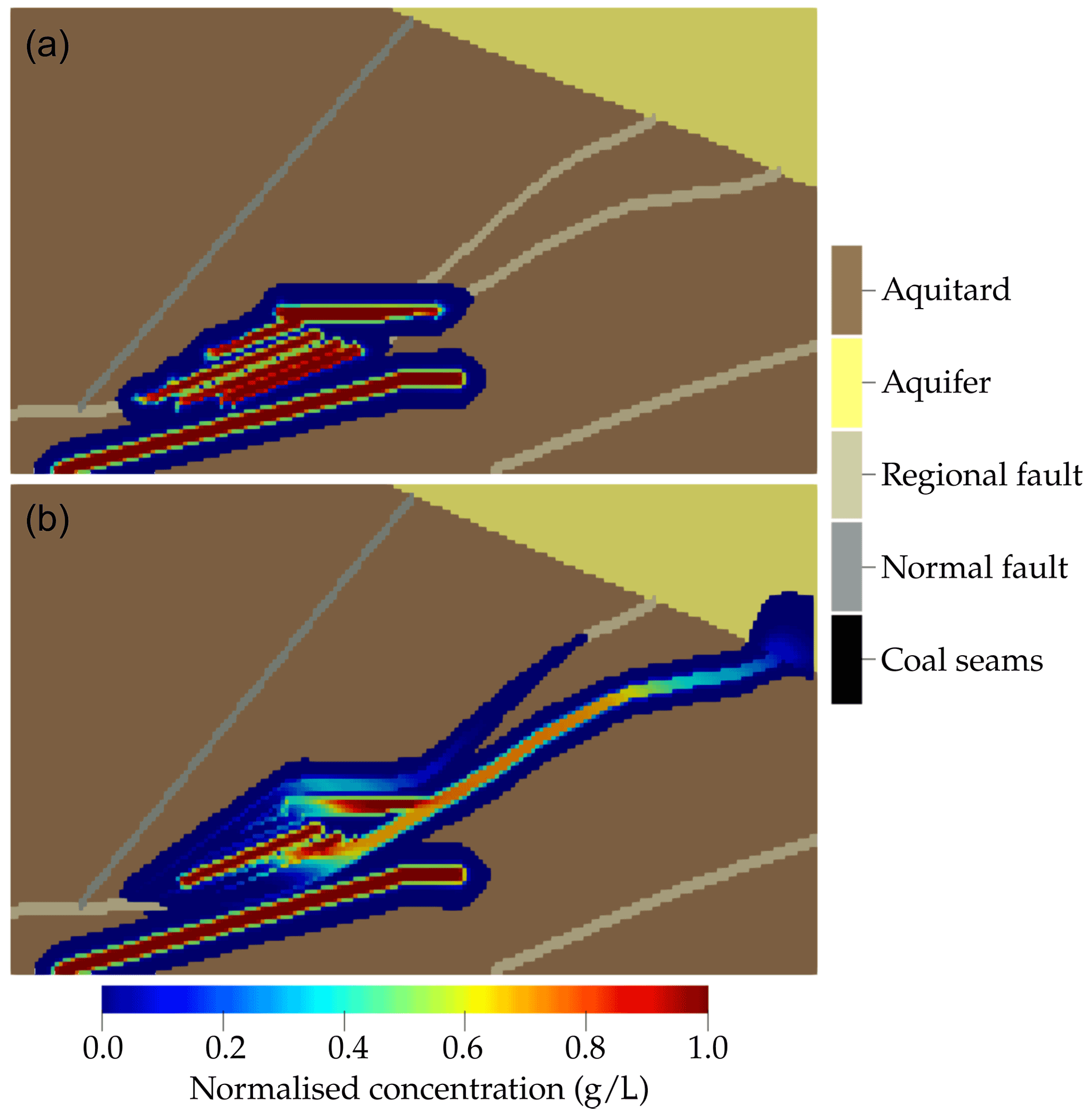
Figure 6 Concentration distribution after 50 years for (a) minimum and (b) maximum hydraulic conductivity of the regional faults.

The topographically-driven pressure head assigned to the left model boundary is also of major importance: contaminants mainly remain in the in situ conversion reactors if a constant lateral pressure head is applied, representing a constant water table along the entire lateral model dimension. In this case, neither density-driven advection nor diffusion can induce any significant contaminant migration towards the fresh water aquifer. In contrast, the maximum lateral pressure head difference of 1.7 MPa accelerates the contaminant migration along the respective fault zones. However, the contaminants still do not arrive in the fresh water aquifer after a simulation time of 50 years.

In case of retardation, contaminant migration is significantly lower. If all layers and fault zones are parametrised with the average retardation coefficient of five, the progress of the contaminant front does not even achieve half of that in the reference case which completely neglects retardation. Also the contaminant concentrations found in the fault zones are considerably lower. For the maximum retardation factor of nine, identical effects are observed in a slightly more pronounced form. Especially retardation within the fault zones strongly reduces the probability of contaminant arrival in the freshwater aquifer.

The hydraulic conductivity of the aquifer becomes mainly relevant if the fault zones have a high hydraulic conductivity. With regard to the reference case, there is no difference when the minimum or maximum values of hydraulic conductivity is chosen. In contrast, these differences become substantial when the hydraulic conductivity of the regional faults is increased to its maximum: a low hydraulic aquifer conductivity does not lead to a contaminant arrival in the fresh water aquifer after 50 years of simulation as it is the case for the average hydraulic aquifer conductivity. On the other hand, a higher hydraulic aquifer conductivity increases contaminant concentrations and flow velocities, so that after 50 years of simulation time contaminants arrive along two regional faults instead of just one. Although the size of the contaminant plume is only slightly affected, maximum concentrations in the aquifer increase to 0.3 g L⁻¹ (30 % of the source concentration).

In the worst-case scenario with the hydraulic conductivities and lateral pressure differences set to their maximum and retardation to its minimum, high contaminant concentrations are observed in the fresh water aquifer. After a simulation time of 30 years, a contaminant plume with more than about 5 % of the total contaminant mass has entered the fresh water aquifer (Fig. 7, top). After a simulation time of 50 years, about 32 % of the total contaminant mass is observed in the fresh water aquifer, and concentrations along the fault zone are already decreasing (Fig. 7, bottom). Hereby, maximum concentrations observed in the fresh water aquifer amount to about 70 % of the initial source concentration. Besides the middle and upper regional faults, contaminants may also migrate along the lower regional fault. From the in situ coal conversion reactors located in the lowest coal seam, contaminants are widely spread across the aquitard, especially towards the lower fault. In contrast, contaminant migration along the normal fault at the left is not observed.

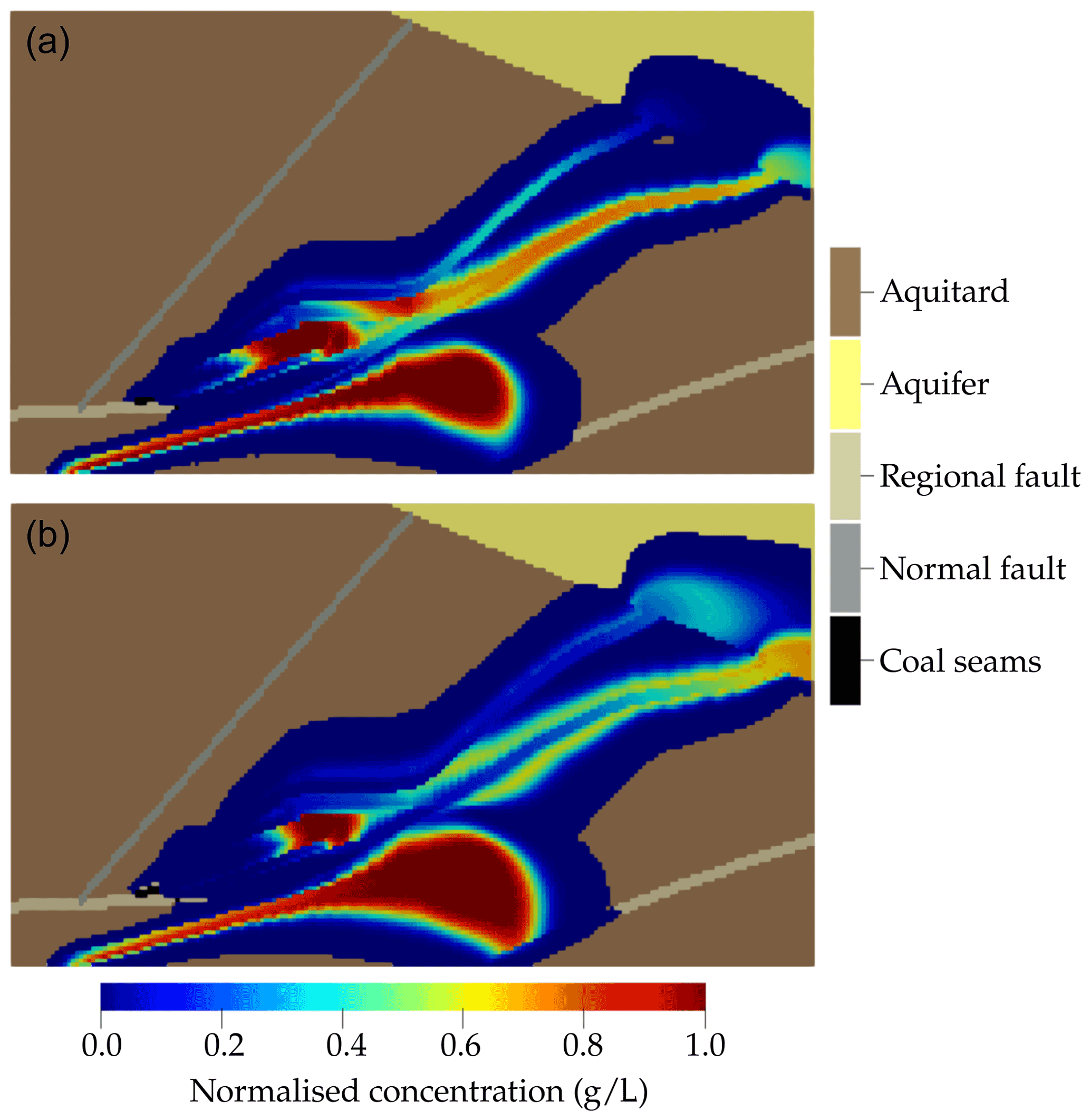
Figure 7 Simulated contaminant concentration distribution for the worst-case scenario with all hydraulic conductivities and the lateral pressure head set to their maximum values and retardation neglected after simulation times of 30 years (a) and 50 years (b).

To examine the influence of retardation in further detail, the worst-case scenario was also simulated under consideration of average and maximum retardation factors. In both cases, contaminants migrate further than in the reference case, but do not reach the fresh water aquifer. The concentration distributions correspond well with the worst-case scenario after simulation times of 5–10 years. Accordingly, it has to be expected that the aquifer will be contaminated as well at a later simulation time. Nevertheless, the increased arrival time may also increase the relevance of contaminant degradation, e.g., due to chemical or biological processes.

3.2 Parameter Correlation Analysis

Figure 8 shows the distribution of input parameters against the maximum contaminant concentration in the freshwater aquifer, whereby the initial source concentration amounts to 1.0 g L⁻¹.

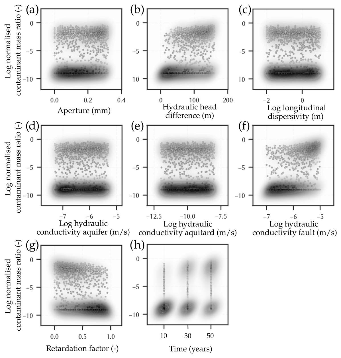
Figure 8 Distribution of all input parameters of the thermo-hydrogeological model of the Máza-Váralja study area against the output contaminant mass ratio in the aquifer with kernel density estimations of the points (shades): (a) fracture aperture, (b) lateral hydraulic head difference, (c) longitudinal dispersion length, (d) hydraulic aquifer conductivity, (e) hydraulic aquitard conductivity, (f) regional fault hydraulic conductivity, (g) retardation coefficient, and (h) simulation time.

The output data is bimodally distributed with distinct peaks at 1 × 10⁻⁹, and 1 × 10⁰ g L⁻¹, corresponding to the minimum and maximum concentration values in the data set. Biomodal characteristics are expected for contaminant transport through fractured media, where species transport by hydrodynamic dispersion plays only a minor role compared to advection. If the source concentration remains constant over a certain time period, the contaminant plume is mostly displaced, and it either reaches the aquifer or not, depending on the initial and boundary conditions.

Nevertheless, some clear correlations can be derived from the kernel density of the points and the bivariate correlation heatmaps (Fig. 9): positive correlations are found for the lateral hydraulic head difference, hydraulic fault conductivity and simulation time, which are reasonable. A negative correlation is observed for the retardation coefficient, since this parameter is reducing contaminant migration with increased values. The QMC sampling of the input parameter space results in the absence of any correlation between the single input parameters, as initially designed and intended.

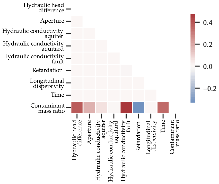
Figure 9 Heatmap for the input parameters and contaminant mass ratio in the fresh water aquifer showing Pearson's correlation coefficients for each parameter ensemble.

4 Summary and Conclusions

The 2D thermo-hydrogeological simulation results for the Máza-Váralja coal deposit show that the regional faults represent the main contaminant migration pathway for this hydrogeological system. The contaminant mass ratio in the freshwater aquifer shows a bimodal distribution with distinct peaks corresponding to the minimum and maximum contaminant source concentrations. For contaminant transport via faults, this can be expected since hydrodynamic dispersion plays a minor role compared to advection, only. If the contaminant source concentration stays constant, the plume is mostly displaced, and thus triggers aquifer contamination or not. Thus, the probability of groundwater contamination mainly depends on the fault hydraulic conductivity, which is recommended to be investigated in more detail in combination with the local lateral pressure gradient. The presented results are valid for the investigated simulation time of 50 years, which exceeds the legally prescribed post-operational monitoring period for recovery and resolution of abandoned mining sites. The simulations undertaken here serve as a preliminary scoping investigation, identifying the most important parameters to be considered in a detailed 3D numerical simulation study requiring additional field data, e.g. hydraulic testing of fault systems.

Nevertheless, from the analysis of the 2D thermo-hydrogeological simulation results, the following conclusions can be made.

The sensitivity analysis shows that extreme cases of groundwater contamination within a simulation time of 30–50 years only occur if the hydraulic conductivity of the regional faults equals the maximum value of 10⁻⁵ m s⁻¹. In addition to that, minimum lateral pressure gradients and low retardation coefficients are required for that purpose. The hydraulic conductivity of the aquifer is important as well. Here, at least an average value of 5 × 10⁻⁷ m s⁻¹ is necessary to induce a contamination in the hydrogeological system. Its influence increases with the hydraulic conductivity of the regional faults.

In case of low hydraulic conductivities of the regional faults and the fresh water/aquifer or a retardation factor above one, contaminant migration is reduced but present. Accordingly, it has to be considered that the contaminants will arrive in the fresh water aquifer at a later time. In contrast, the absence of a topgraphically-driven pressure gradient causes the contaminants to remain in the in situ conversion reactors, which is also observed for the simulations with minimum hydraulic conductivities assigned to the regional faults (10⁻⁷ m s⁻¹).

The hydraulic aquitard conductivity is of minor importance. Here, high hydraulic conductivities increase the contaminant plume distribution within the aquitard but not its migration distance towards the aquifer. Migration along other regional faults than the middle one is increased, but the normal fault in the left model area is not reached by the contaminants. This is of high relevance because its conductivity is expected to be up to two orders of magnitude higher than that of the regional faults. Transport along the normal fault would thus considerably increase the probability of any fresh water aquifer contamination.

The worst-case scenario shows that significant contamination of the aquifer is feasible under specific geological conditions, i.e. maximum hydraulic conductivities and lateral pressure gradient. Thereby, more than 30 % of the contaminant mass migrate into the fresh water aquifer within a simulation time of 50 years and reach about 70 % of the initial source concentration. Under these circumstances, retardation becomes especially relevant as it delays contaminant migration and provides more time for chemical or biological degradation processes.

The presented sensitivity analyis was employed to develop a web-based and interactive Environmental Hazards and Risk Management Toolkit (EHRM) to allow for an integrated risk analysis of the application of in situ coal conversion by Tranter et al. (2022).

The EHRM toolkit uses four different surrogate strategies to integrate the results of the thermo-mechanical (Hedayatzadeh et al., 2022) and hydrogeological numerical simulations undertaken in the higher-level interdisciplinary study. Tranter et al. (2022) present its application to two European coal regions.