 | 18 May 2022
Portable two-filter dual-flow-loop 222Rn detector: stand-alone monitor and calibration transfer device
Alan D. Griffiths
Alastair G. Williams
Ot Sisoutham
Viacheslav Morosh
Stefan Röttger
Florian Mertes
Annette Röttger
Little overlap exists in the required capabilities of 222Rn (radon) monitors for public health and atmospheric research. The former requires robust, compact, easily transportable instruments to characterise daily to yearly variability >100 Bq m−3, whereas the latter requires static instruments capable of characterising sub-hourly variability between 0.1 and 100 Bq m−3. Consequently, detector development has evolved independently for the two research communities, and while many radon measurements are being made world-wide, the full potential of this measurement network can't be realised because not all results are comparable. Development of a monitor that satisfies the primary needs of both measurement communities, including a calibration traceable to the International System of Units (SI), would constitute an important step toward (i) increasing the availability of radon measurements to both research communities, and (ii) providing a means to harmonize and compare radon measurements across the existing eclectic global network of radon detectors. To this end, we describe a prototype detector built by the Australian Nuclear Science and Technology Organisation (ANSTO), in collaboration with the EMPIR 19ENV01 traceRadon Project and Physikalisch-Technische Bundesanstalt (PTB). This two-filter dual-flow-loop radon monitor can be transported in a standard vehicle, fits in a 19′′ instrument rack, has a 30 min temporal resolution, and a detection limit of ∼0.14 Bq m−3. It is capable of continuous, long-term, low-maintenance, low-power, indoor or outdoor monitoring with a high sensitivity and an uncertainty of ∼15 % at 1 Bq m−3. Furthermore, we demonstrate the successful transfer of an SI traceable calibration from this portable monitor to a 1500 L two-filter radon monitor under field conditions.
- Article
(4406 KB) - Full-text XML
-
Supplement
(279 KB) - BibTeX
- EndNote


1.1 Background
The unique physical characteristics of 222Rn (radon) make it a health risk as well as a powerful tracer of atmospheric mixing and transport processes. As such, it has long been a species of interest to the radiological protection, air quality and climate change research communities. Direct health risks associated with radon have been documented for around 500 years (Jacobi, 1993), and it is still responsible for about half of the radiation dose to most people. Consequently, the identification of high radon priority areas is an ongoing concern, and the World Health Organisation recommends mitigation if there is risk of prolonged exposure in dwellings or workplaces to radon concentrations exceeding 100 to 300 Bq m−3 (WHO, 2009; see also BSSD, 2013; IAEA SSS, 2015) Regarding indirect risks, near surface radon, and the washout of radon progeny, constitute a large source of uncertainty in radiological emergency early warning networks (Melintescu et al., 2018).
Shortly following its formal discovery in 1898, radon was recognised as a powerful tracer of terrestrial influences on air masses (Satterly, 1910; Wright and Smith, 1915). Radon's utility as a tracer of vertical mixing has been demonstrated through numerous surface-atmosphere exchange (Moses et al., 1960; Hosler, 1968; Kirichenko, 1970; Fontan et al., 1979; Fujinami and Osaka, 1987; Porstendörfer, 1994; Williams et al., 2011, 2013) and urban pollution/urban climate (Perrino et al., 2001; Sesana et al., 2003; Kikaj et al., 2020; Chambers et al., 2019b) studies. Its efficacy as a tracer of long-distance transport has been demonstrated in studies seeking to characterise multi-annual trends in hemispheric-mean values of greenhouse gases (GHGs) and ozone depleting substances (Williams and Chambers, 2016; Chambers et al., 2016). Furthermore, the combination of radon's unique physical characteristics makes it a valuable tool for evaluating the mixing and transport schemes of regional- to global-scale chemical transport models (Zhang et al., 2008; Locatelli et al., 2014; Chambers et al., 2019a; Zhang et al., 2021), for improving the accuracy of regulatory dispersion modelling, and providing a top-down constraint on local- to regional-scale emissions of GHGs using the radon tracer method (Levin et al., 1999, 2021; Grossi et al., 2018).
Within the atmospheric boundary layer (ABL), average radon concentrations for inland regions typically vary between 5 and 15 Bq m−3. As radon emissions move upwards away from their source at the terrestrial surface, concentration drops across the daytime surface layer (∼100 m) are typically <0.5 Bq m−3 (Chambers et al., 2011; Levin et al., 2020). In contrast, at night strong thermal gradients can trap large amounts of radon near the surface leading to strong gradients across the nocturnal inversion (located at heights of ∼20–200 m a.g.l., depending on local meteorological and geographical conditions). Throughout the remainder of the ABL/Residual Layer above, vertical changes are generally small due to vigorous mixing within thermals during the day followed by quiescent conditions at night. In the free troposphere above the ABL, radon concentrations can reduce to 0.01 Bq m−3 or less (Liu et al., 1984; Kritz et al., 1998; Williams et al., 2011). In the remote marine boundary layer, on the other hand, mixing in the absence of a significant surface radon source tends to result in minimal vertical radon gradients, and concentrations can fall below 0.05 Bq m−3 (Balkanski et al., 1992; Polian et al., 1996; Zahorowski et al., 2013; Chambers et al., 2018).
Clearly, the concentrations at which radon is considered a health risk, and those at which it is typically employed as a tracer in atmospheric research, vary by orders of magnitude. Consequently, measurement techniques employed by the different research communities have evolved quite independently, driven by vastly different requirements. Since high concentrations and extended exposure are of most concern to public health, portability, low cost, and ease of operation for daily to yearly timescales have been the primary development considerations. By contrast, highly sensitive monitors (0.01 to 100 Bq m−3) with fast response times (10 to 60 min) have been the primary goal for atmospheric and environmental applications.
A complaint common to all radon-related research communities is that more radon measurements are required globally to help constrain their respective problems. With this need in mind, increasing the number, traceability, and accessibility of radon observations across Europe is a key goal of the EMPIR 19ENV01 traceRadon Project (Röttger et al., 2021). Potentially, this goal could be achieved faster with a radon detection system that is usable in multiple contexts. To address this need, we introduce a portable radon monitor capable of long-term autonomous operation, 30 min temporal resolution, with the ability to reliably measure radon concentrations within the range 0.1 to 1000 Bq m−3 for which a calibration traceable to the International System of Units (SI) has been developed. We also demonstrate its suitability to be used as a calibration transfer device to harmonise radon measurements across monitors in the European measurement network (Whittlestone and Zahorowski, 1998; Perrino et al., 2001; Levin et al., 2002; Schmithüsen et al., 2017; Grossi et al., 2020), and globally (Pereira, 1990; Wada et al., 2010).
For over twenty years the two-filter dual flow-loop technique has provided the most sensitive, high temporal resolution radon observations in the world (Whittlestone and Zahorowski, 1998; Williams and Chambers, 2016; Chambers et al., 2018), despite the hitherto lack of a calibration traceable to the SI. Introduction of a second flow-loop to earlier two-filter detector designs (Thomas and Leclare, 1970; Schery et al., 1980; Whittlestone, 1985) and improving the efficiency of the sensing head have resulted in the most significant improvements. However, since the detection limit (DL) of the two-filter dual flow-loop technique is inversely proportional to detector size (volume), to date, these instruments have not been readily portable. This has posed significant logistical challenges for installation at remote sites and limited their uptake for environmental research applications.
1.2 State-of-the-art in contemporary atmospheric radon detection
A variety of commercial “active” radon monitors (capable of resolving diurnal changes) have been developed for public health studies (Table 1) but reported DLs of the leading commercial detectors are between 2 to 4 Bq m−3. Through a combination of radon's terrestrial source and daily changes in ABL depth, the diurnal cycle of radon at typical inland sites is characterised by a morning maximum between 10 and 50 Bq m−3 and afternoon minimum between 0.5 and 2 Bq m−3. As such, outdoor radon concentrations are often below the DLs of commercial radon detectors for 30 %–40 % of each day.
Table 1A selection of contemporary radon monitors in order of their reported sensitivity to 222Rn.

Two kinds of non-commercial (i.e., “research grade”) active radon monitors have been developed to satisfy the high-sensitivity and high-temporal-resolution requirements of outdoor monitoring: (i) “indirect” monitors, which sample ambient radon progeny, and (ii) “direct” monitors which sample ambient radon gas. Indirect monitors use a single filter to collect ambient radon progeny (for α or β counting) as a proxy for radon concentration (e.g., Schmithüsen et al., 2017; Perrino et al., 2001). While these instruments are fast and compact, the relationship between radon and its progeny (the “equilibrium factor”) changes with height in the lowest 50 to 100 m of the ABL (Jacobi and André, 1963). The measurement may be further influenced by the ambient aerosol loading, the atmospheric mixing state, humidity, rainfall, and tube loss effects (Levin et al., 2017). Consequently, while high-precision relative changes in radon concentration can be reported by these monitors under most conditions, calibration traceability can be problematic. By contrast, direct radon monitors operate by first removing all ambient radon progeny and allowing only radon gas and aerosol-free air to enter a delay chamber. Within this chamber, new progeny form under controlled conditions, which are then captured and counted (with varying degrees of efficiency depending on detector design). The requirement of a sample delay chamber makes direct radon monitors larger than indirect monitors and increases their response time. However, the calibration traceability of direct radon monitors is generally less problematic. For this reason, direct radon monitors are the main focus of Table 1, in which instruments have been ranked according to their reported sensitivity. Further detail regarding indirect monitors can be found in Schmithüsen et al. (2017).
The measurement uncertainty of a radon monitor is influenced by: (i) the counting uncertainty, (ii) instrumental background characterisation and removal, (iii) the accuracy of the calibration source, (iv) accuracy of the calibration method, (v) requirements for conditioning of sample air (e.g., drying in the case of electrostatic deposition monitors). For radon concentrations typical of the outdoor atmosphere, the counting uncertainty of a well-maintained instrument usually constitutes the largest fraction of the absolute uncertainty. For remote oceanic or high elevation sites, characterised by very low concentrations, the instrumental background becomes increasingly important. Together, the counting uncertainty and background have the largest influence on a monitor's DL. Since background information was not available for all instruments in Table 1, DLs have only been included for some monitors. Clearly, with sensitivities 1–2 orders of magnitude greater than commercial monitors (Table 1), only research-grade radon monitors can provide reliable, representative radon concentration estimates across the diurnal cycle year-round at most sites.
At the time of writing this report, the most sensitive demonstrated radon measurements (DL 0.0016 Bq m−3) had been made by Choi et al. (2001), using an electrostatic deposition monitor. However, this sensitivity was achieved by integrating measurements over a 24 h period. The most sensitive high-temporal-resolution radon measurements have been made by the unique 5000 L ANSTO two-filter dual flow-loop detector currently operating at the Cape Grim Baseline Atmospheric Pollution Station (Williams and Chambers, 2016). The DL of this instrument is between 0.005 and 0.01 Bq m−3 for hourly observations. However, the most sensitive readily available research-grade direct radon monitor is the 1500 L ANSTO two-filter dual-flow-loop detector, of which there are currently 32 in operation world-wide. This instrument has a DL of ∼0.025 Bq m−3, is weatherproof, has low maintenance requirements, a 45 min response time (correctable in post processing; Griffiths et al., 2016), is remotely controllable, and is automatically calibrated in situ. However, this monitor has a footprint of 3.0×0.9 m2, weighs ∼120 kg, and requires a separate 370 W stack blower to maintain its 80 to 100 L min−1 sampling rate. A truck is required to move it, and 4 people (or a mechanical aid) to lift it into position.
1.3 Aims and scope
Our goal was to develop a portable two-filter dual flow-loop radon monitor that could be traceably calibrated, easily deployed (either for long-term stand-alone use, or campaign-style as a calibration transfer reference device) and suit the primary needs of both the radiation protection and atmospheric science radon research communities. Design constraints required: (i) the monitor to be transportable with minimal disassembly by one person in a standard vehicle; (ii) quick and easy setup; (iii) vertical orientation to minimise its footprint and enable maintenance access from above; (iv) suitability for indoor or outdoor deployment, and (v) a DL <0.2 Bq m−3. Here we introduce a prototype of the portable detector, summarise the traceable calibration method, demonstrate its performance in the field at low radon concentrations, and use it to transfer a calibration to a 1500 L model two-filter detector under field conditions.
2.1 Overview and principle of operation
In principle, two-filter dual flow-loop radon detectors operate as follows: ambient aerosols, radon progeny and thoron (220Rn) are removed from the sampled air, which then passes directly into a delay chamber as part of the first flow loop (the “external” or sampling flow loop). New radon progeny form in the delay chamber under relatively controlled conditions. A second flow-loop (the “internal” flow loop) repeatedly draws this air through a second filter inside the delay chamber, which captures the newly formed progeny for counting. α-decays of the short-lived 218Po and 214Po on this filter are counted using a zinc sulphide/photomultiplier tube (ZnS-PMT) assembly (henceforth referred to as the “measurement head”), and the 30 min α-count rate related to a radon activity concentration (by calibration with a known source).
In practice, many factors need to be considered to ensure optimal performance.
Sampling rate. Sample residence time in the delay chamber influences both the detector response time and the isotope selectivity (discussed below). Ideally, the ratio of delay chamber volume (L) to sample flow rate (L min−1) should be maintained at a relatively consistent value between 15 and 20 min. The opposing portability and DL constraints limited the size of the delay chamber to 200 L, for which the appropriate sampling rate is between 10 and 14 L min−1.
Instrumental background. Background counts are contributed to by: (i) accumulation of 210Pb (T0.5 22.3 years) on the second filter, (ii) cosmic radiation, (iii) radiation from the surrounding soils, rocks and building materials, and (iv) self-generation of radon inside the detector from trace amounts of 226Ra. Although typically small, and relatively constant on monthly to quarterly timescales, contributions (ii) and (iii) above are location dependent (requiring background estimates to be confirmed in situ). Provided no soil dust is permitted to enter the detector during maintenance periods, contribution (iv) is also relatively constant (226Ra half-life = 1600 years). 210Pb accumulates gradually on the second filter and can typically be approximated using a linear model (see Sect. 2.3). The rate of this accumulation depends on the long-term average radon concentration to which the detector is exposed (including calibration events).
Radon isotope selectivity. The measurement head provides a gross α-count, with no ability to distinguish α-particles from non 222Rn progeny. To ensure 222Rn-specific detection, other radon isotopes (e.g., thoron: 220Rn, T0.5 55.6 s; and actinon: 219Rn, T0.5 4 s) need to be eliminated. This is achieved, to a reasonable accuracy, by incorporating a “dead volume” in the inlet line to delay the air by ∼5 220Rn half-lives. This is referred to as the “thoron delay”. 220Rn and 219Rn progeny that form in the thoron delay are removed by the detector's first (primary) filter, ensuring only aerosol-free air and 222Rn gas enter the detector's delay chamber.
Protecting the primary filter. If radium-containing aerosols (e.g., soil dust) collect in the primary filter (or thoron delay), this constitutes a separate source of 222Rn and 220Rn directly at the inlet of the detector's delay volume. Since the primary filter (a Luwa JK Ultrafilter; https://pdf.directindustry.com/pdf/luwa-air-engineering-ag/luwa-ultra-filter-jg-jk-jp/25860-267455.html, last access: 18 May 2022) is relatively expensive and non-trivial to replace, a disposable coarse particle filter is installed upstream of the thoron delay to protect the primary filter.
Minimising plate-out and decay losses. The second flow-loop needs to be fast enough for the entire volume of air in the delay chamber to pass through the second filter approximately once per minute. This high flow rate is required for two reasons: (i) the half-life of radon's first α-emitting progeny (218Po) is short (3.1 min), and (ii) to minimise the time for plate-out of unattached radon progeny on the internal surfaces of the detector. High flow rates, however, are usually also associated with strong turbulent mixing, which can increase plate-out losses. To approximate laminar (or plug-like) flow to the measurement head along the length of the detector's delay chamber, air in the second flow-loop is passed through a flow homogenising screen.
Power consumption and maintenance. Excluding ambient aerosols from the delay chamber ensures that newly formed radon progeny remain unattached to aerosols (Porstendörfer et al., 2005). As such, they can be captured efficiently on a relatively open weave metal mesh filter (635 mesh, TWP Inc.) as opposed to a more traditional glass fibre filter. This filter (a twill weave stainless steel mesh consisting of 20 µm diameter wire with 20 µm openings) has a very low flow impedance, enabling high flow rates to be sustained with a low power (21 W) centrifugal blower (PAPST RG160-28/12N; http://www.ebmpapst.com, last access: 18 May 2022), which typically runs continuously, maintenance-free, for over 10 years. The low sampling flow rate required for this monitor enables the same model of blower to be used to drive the sampling flow loop when measuring near the surface. The overall power consumption under normal operation can thus be limited to ∼100 W.
Compatibility. A variety of research-grade radon monitors, based on different measurement principles and different instrumental response times, operate at monitoring network stations globally. Some report radon concentrations corrected to STP (e.g., the HRM, Levin et al., 2002; 1000 hPa, 20 ∘C), while others (e.g., Tositti et al., 2002; Wada et al., 2010; Grossi et al., 2012) report radon activity concentration in dry air. For greatest compatibility with other observed and simulated radon concentrations, two-filter dual flow-loop radon monitors measure the temperature, relative humidity, and pressure in the delay volume to enable retrospective STP correction and calculation of dry air mixing ratios. A deconvolution algorithm is also available to correct for the instrument's response time (Griffiths et al., 2016; see also Sect. 3.1).
A schematic of the 200 L radon monitor (henceforth referred to as “the reference monitor”, due to its intended use as a calibration transfer standard device) is presented in Fig. 1. The detector, constructed of marine-grade stainless steel, consists of two stackable pieces: the thoron delay, and the main detector. The main detector consists of two inseparable compartments: the delay chamber and an electronics enclosure.
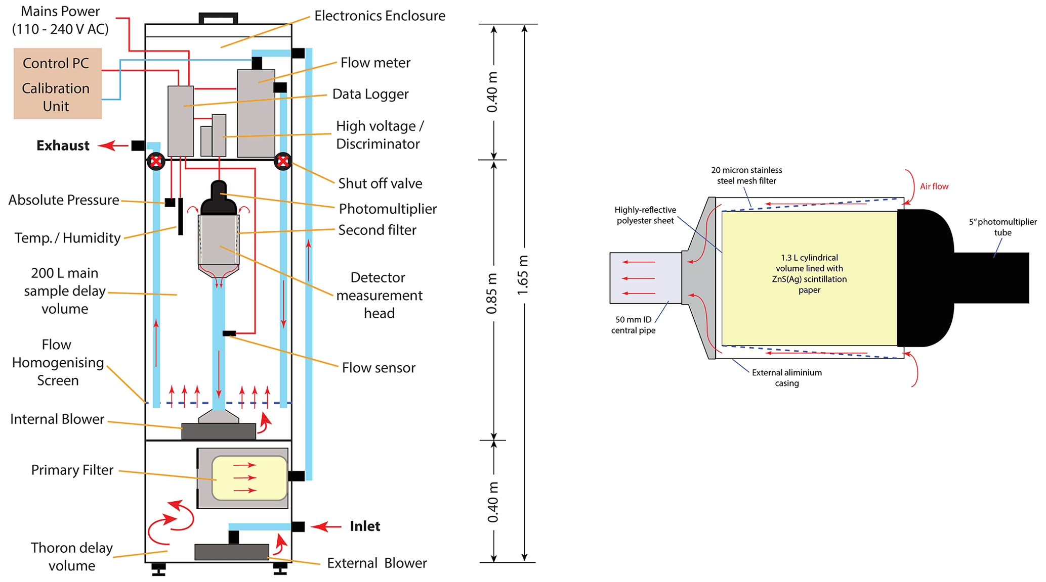
Figure 1(a) Schematic of the reference monitor, and (b) schematic of the monitor's radon measurement head.
The detector's footprint was restricted to 0.48×0.48 m2 to enable it to fit in a 19′′ instrument rack. A relative size comparison with larger models of two-filter radon monitor is provided in Fig. 2.
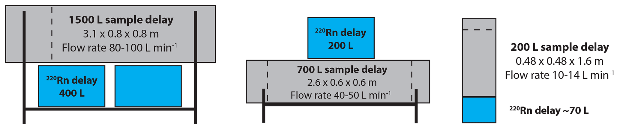
Figure 2Size comparison (to scale), of three models of ANSTO two-filter dual flow-loop atmospheric 222Rn monitors.
The external flow-loop blower and primary filter are in the thoron delay, which has a total volume of 92 L, but an active mixing volume of ∼70 L. If a long sampling line is required (e.g., >20 m), a separate stack blower (e.g., SV5.90/2 0.37 kW; Becker) may be necessary to achieve a suitable, stable flow rate, because the PAPST blowers are not powerful and flow impedance can become significant for long sampling lines of diameter 20 mm (standard for this monitor). Wind speed also increases away from the surface, such that the venturi effect can cause large fluctuations in flow rate when sampling from tall towers if underpowered blowers are used. Since radon is unreactive, the specific type of inlet line is not critical, but high or medium density polyethylene pipe is recommended since it is durable, UV resistant, and comes in continuous lengths (so joins can be minimised, which is crucial if the inlet line needs to be buried).
The external flow-loop blower draws air from the sampling point into the thoron delay, generating an overpressure that pushes the delayed air through the primary filter. The conditioned air then passes, via an external pipe, to a volumetric flow meter (ABB Metering Pty Ltd model DS5 http://new.abb.com, last access: 18 May 2022), prior to entering the bottom of the delay chamber, behind the flow homogenising screen. The internal flow-loop blower draws air from the top of the delay chamber through the second filter in the measurement head and returns this air to the bottom of the delay chamber via a central 50 mm PVC pipe. The homogenising screen in this flow-loop results in a pressure gradient along the delay chamber of 100 to 150 Pa, which helps sampled air to exit the delay chamber via the exhaust line. A valve is located at the end of the exhaust line that can be constricted to maintain an overpressure at the top of the delay chamber (relative to ambient) of 100 to 200 Pa, to minimise the chance of any near-surface external air directly entering the detector should any leaks develop.
The second filter in the measurement head is angled at approximately 5∘ to the air flow (Fig. 1b). While the 20 µm openings of the mesh filter are large compared with the diameter of the unattached radon progeny, the charged particles are highly mobile and attach to the mesh with high efficiency. The mesh surrounds a 1.3 L cylindrical volume, the outer surface of which consists of clear polyester sheet coated with silver activated zinc sulphide (SGC-200-1475, DTect Innovation Pty. Ltd.) supported by an aluminium frame. The angled mesh filter is maintained at a distance of between 1–7 mm from the ZnS(Ag) to minimise the number of α-particles stopped in air prior to impacting the ZnS(Ag). A proportion of the α-particles emitted by the captured 222Rn progeny strike the ZnS(Ag), resulting in fluorescence. Technically, α-particles from radon decay can also directly contribute to observed counts, but this is only possible for radon atoms that decay while inside the small volume between the detector head casing and the scintillation material (Fig. 1b), assuming their α-particles are emitted in the direction of the scintillation material and are not stopped by the mesh filter. In practice, this contribution is very small.
The bottom of the head volume is coated with a highly reflective polyester film to reflect light emitted in that direction back to the top, an open viewing window for a 5′′ photomultiplier tube (9330B, ET Enterprises). The capture and counting efficiency of the head is accounted for in the calibration procedure (see Sect. 2.4). In contrast to the larger model detectors, the measurement head in the reference monitor is mounted vertically and held securely in place with a padded collar. As such, the reference monitor can be operated on moving platforms more reliably and transported between sites without the need to remove the delicate measurement head.
For short-term (weeks-to-months, “campaign-style”) use, the reference monitor can be calibrated prior to deployment, and the monitor can run completely autonomously requiring only mains power (∼140 kB data per month, 8 MB of logger memory). All data is stored in the non-volatile (but circular) memory of the internal Campbell Scientific data logger. For longer-term deployments (years to decades), a controlling computer is connected to the logger via serial link or Bluetooth. Monitoring software on the computer downloads data from the logger every 30 min to small (∼140 kB) monthly data files and enables remote access to the data stream, as well as full remote control of a separate calibration and background module, which can be connected to the monitor via a USB link and 4 mm tubing.
The compact nature of the reference monitor, compared to the larger models, enables it to fit inside a large (e.g., 20 m3) controlled climate chamber of the kind operated by Physikalisch-Technische Bundesanstalt (PTB, Braunschweig, Germany). This has enabled an SI traceable calibration to be developed for a two-filter dual flow-loop radon monitor for the very first time (see Sect. 2.4). Furthermore, the low sampling flow rate enables field calibration and background estimates to be made using radon-free compressed gas, rather than having to calibrate on top of the ambient sampling flow, substantially reducing uncertainty compared with existing two-filter monitors.
2.2 Construction and commissioning tests
Small differences in the quality of consumable materials (i.e., filter mesh and scintillation paper), and tolerance of electronic components, result in a unique set of characteristics for each detector. The most important characteristic to determine for each new (or refurbished) detector is the “working voltage” (WV); i.e., the high voltage (HV) supplied to the PMT. The WV is determined through joint optimisation of the background and detector sensitivity to radon.
At a given time and location, the background count changes as a function of the HV supplied to the PMT (Fig. 3a). For a given radon concentration, the same is true of the detector's sensitivity (Fig. 3b). Temperature sensitivity of the electronic components that comprise the PMT power supply can result in diurnal and seasonal variability in the nominally constant HV supplied to the PMT of amplitude between 1 and 10 V. Consequently, the first consideration for the WV is for it to be within a range of HV settings for which the detector's rate of change in sensitivity with HV is low (e.g., between 650 and 725 V, Fig. 3b). Of the HV settings well within this range (e.g., 675 to 700 V), the voltage yielding the lowest instrumental background should be chosen. Based on the characteristics shown in Fig. 3, a WV of 675 V is most appropriate for this particular monitor.

Figure 3Example (a) instrumental background, and (b) sensitivity response, as a function of HV supplied to the counting assembly at a constant radon concentration (in this case 190 Bq m−3).
For ANSTO-built radon monitors the DL is arbitrarily defined to be the radon concentration at which the relative counting error reaches 30 %. Based on the background and sensitivity information provided in Fig. 3 (valid for one point in time, usually when the detector is assembled or first commissioned), it is possible to estimate the relative counting error at each HV setting for a range of hypothetical radon activity concentrations (see Chambers et al., 2014, for details). Assuming a working voltage of 675 V, Fig. 4 indicates that the reference radon monitor has a detection limit of ∼0.14 Bq m−3. To keep abreast of the detector's performance, it is important to regularly monitor the instrumental background and detector sensitivity (as discussed in the following sections), since they change slowly with time.
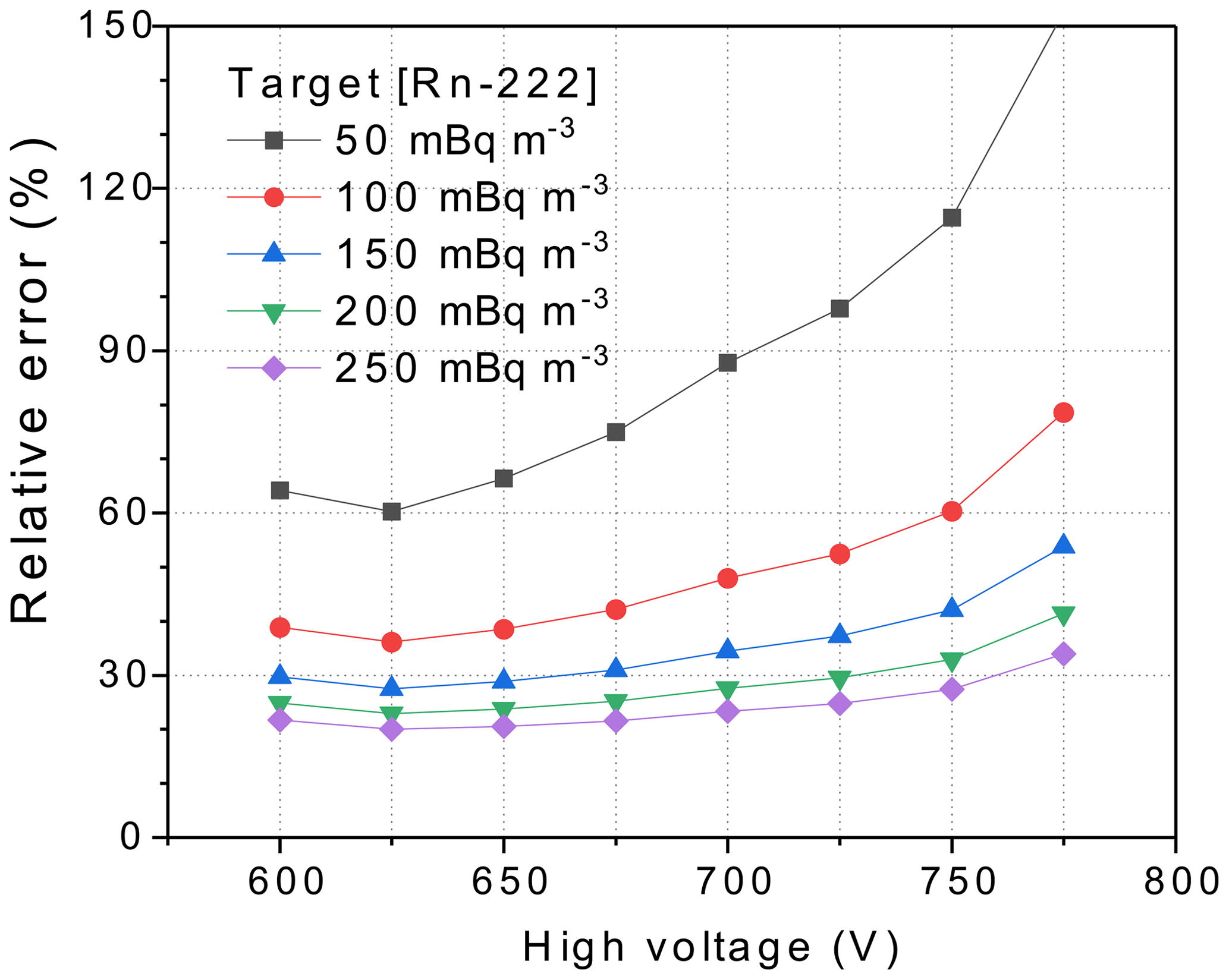
Figure 4Relative counting error as a function of HV for a range of hypothetical radon activity concentrations.
2.3 Instrumental Background Determination
For short (campaign-style) deployments (e.g., ≤3 months), it is sufficient to take the average of background checks before and after the measurement period. For long-term (semi-permanent) installations, however, the background should be checked every 3 months. As shown in Fig. 5, for deployments >6 months, a monitor's background can usually be approximated with a linear model. For optimal detector performance, refurbishment of the measurement head (which includes replacement of the mesh filter and scintillation paper) is recommended when the background count reaches 10 min−1, or every 5 years (whichever comes first), since the integrity of the ZnS(Ag) scintillation material also degrades with time.
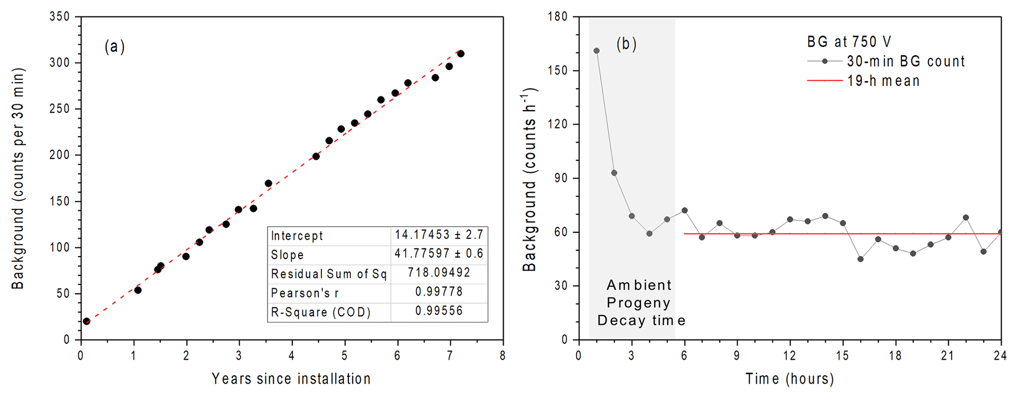
Figure 5Example (a) 7-year background record with linear model, for a 1500 L two-filter dual-flow-loop detector sampling from 2 m a.g.l., ∼55 km inland near Sydney, Australia, and (b) a single 24 h instrumental background check under field conditions. Regarding (a), the annual average radon concentration at this site was 6.8 Bq m−3, afternoon minimums were typically between 0.8–2.2 Bq m−3, and peak nocturnal values in late autumn were 23±σ14 Bq m−3.
For the reference monitor, one of two methods can be used to track changes in the instrumental background:
Method 1. Turn off the external flow loop blower while leaving the internal flow loop blower running. Using a large (e.g., 7.2 m3 at STP) cylinder of radon-free compressed gas (e.g., aged compressed air, or instrument air), establish a flow of 10 L min−1 through the detector for a 12 h period. Given radon's 3.8 d half-life, industrial compressed air bottled >1 month ago (i.e., “aged”) would not contain significant amounts of 222Rn. When analysing the resulting 30 min count data, ignore the first 6 h when the delay chamber will be flushing and the initial collection of short-lived radon progeny on the detector's second filter will be decaying. Derive the background estimate from the average of the last 6 h of 30 min counts. The standard error of these values will provide an indication of the uncertainty associated with this background estimate. This method will account for all factors contributing to the instrumental background.
Method 2. If radon-free gas is not available, turn off the internal and external flow loop blowers. Close the detector's inlet valve. Place a flexible seal (e.g., balloon or partially inflated plastic or Teflon bag) over the detector's exhaust valve to relieve pressure changes associated with diurnal changes in temperature and preventing back diffusion of potentially high ambient radon concentrations at night along the exhaust line into the delay chamber. Leave the detector measuring in this state for 24 h (e.g., Fig. 5b). When analysing the results ignore the first 5–6 h, during which time short lived progeny will be decaying on the detector's second filter. The background estimate is then calculated as the average of the last 18 h of 30 min observations. Note that this method will not account for possible of ingrowth of radon from 226Ra inside the detector (since there is no flow of air through the second filter). There may also be a slight dependence of the background estimate on the radon concentration inside the detector at the time that the blowers were shut down.
The contribution of radon ingrowth to the background signal is essentially constant in time. Consequently, if this has been determined once (e.g., by comparing methods 1 and 2), it can be added to future background estimates determined using method 2. The ingrowth contribution will be unique to each instrument, since each batch of material for making components will have unique levels of trace contamination of 226Ra. Tests conducted in the PTB controlled climate chamber on the reference monitor described here indicated that 40 %–45 % of the instrumental background signal of 1.86 min−1 (when the materials in the measurement head quite new), was attributable to radon ingrowth. A background check using method 2 prior to shipping the detector to PTB indicated a value of (1.07±0.139) min−1, which is consistent with this estimate given that ingrowth is unaccounted for.
In post-processing the linear model of instrumental background as shown in Fig. 5a is removed from the raw counts before calibrating the net half-hourly counts to activity concentrations.
2.4 Calibration
The field calibration procedure for two-filter dual flow-loop radon monitors was designed for the larger model detectors (non-portable, with high sampling flow rates), for which calibration on top of the sampling flow was the only option. The procedure involves injecting radon from a flushed, well-characterised calibration source (Pylon Electronics, https://pylonelectronics-radon.com/radioactive-sources/, last access: 18 May 2022) upstream of the flow meter for 5–6 h while the detector operates normally. For a 1500 L detector the sampling rate is ∼90 L min−1 and the source flush rate 0.1 to 0.15 L min−1 (∼0.2 % of the sampling rate). Ideally, aged (radon-free) air is used to flush the source. However, for calibrations during the day, when the atmosphere is well mixed, using ambient air from ≥2 m a.g.l. does not introduce a large uncertainty (typically <0.1 %); but this air needs to be dried to prevent moisture accumulation in the calibration system, which can reduce the source's emanation rate near saturation. Following a calibration injection, it takes ∼5 h for the radon concentration in the detector to return to ambient values (Fig. 6a).
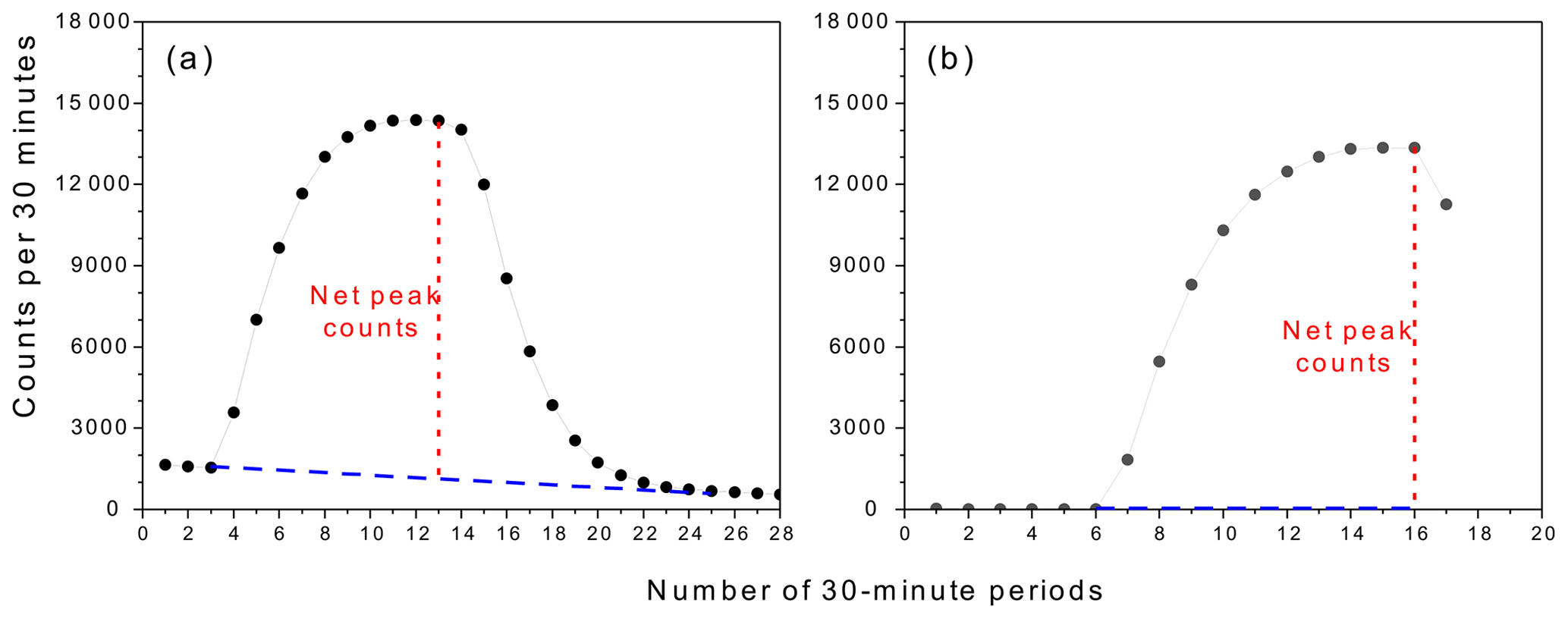
Figure 6(a) Example of a standard field calibration injection on top of the ambient sampling flow, and (b) an example of a calibration injection on a flow of radon-free air.
The detector's calibration factor is determined as the ratio of the net peak count rate at the end of the injection period to the concentration of radon inside the detector (calculated from the radon delivery rate and flow through the detector). Note that for a 5 h injection the net peak count rate should be scaled slightly (by around +1 %) because the radon concentration in the detector would not yet have reached equilibrium. To estimate the net peak count rate it is necessary to assume a linear change in ambient radon over the 10 h calibration period (see dashed blue line in Fig. 6a). This assumption is the largest source of uncertainty in the field calibration process since, unless conditions are windy (well-mixed) or air mass fetch is predominantly over the ocean, ambient radon in the ABL can change substantially over 10 h. The relative uncertainty introduced to the net peak count of Fig. 6a on calm vs. windy days at Lucas Heights (Sydney, NSW) by assuming a linear change in ambient radon over the 10 h calibration window is shown in Fig. 7a.
Because of the uncertainty associated with individual calibration events of the large model detectors, they are usually calibrated monthly (through automatic software scheduling), and then a linear calibration model is developed based on ≥1 year of observations (e.g., Fig. 7b). The scatter about the trend in Fig. 7b is relatively small (±1.5 %), because it is a remote oceanic site with limited local land fetch. For inland sites, the scatter about the long-term calibration trend is typically ±4 % to 6 % (when using a 20 kBq 226Ra source). The larger the source used, the smaller the relative uncertainty in net peak count estimates introduced by diurnal radon variability. Consequently, for detectors monitoring near surface air at inland sites, calibrations are usually performed using 50 to 100 kBq 226Ra sources.
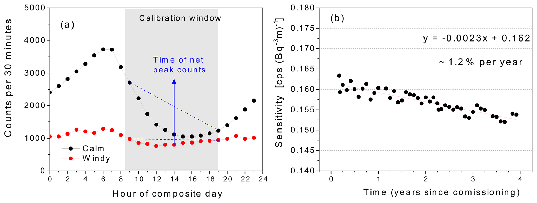
Figure 7(a) Comparison of error in net peak count rate estimate associated with assuming a linear change in ambient radon concentration over a 10 h calibration window on a calm vs. windy day, and (b) example of the deterioration of sensitivity to radon with time for a 700 L two-filter dual flow-loop detector operating at Macquarie Island, in the mid-Southern Ocean.
Linear calibration models for two-filter detectors typically show a consistent (but site dependent) reduction in detector sensitivity of between 0.5 % to 1.5 % per year. This gradual reduction in sensitivity is attributable to the degradation of the consumable materials inside the detector head (i.e., the ZnS scintillation material and 20 µm stainless steel mesh filter), and is largest under humid conditions (e.g., coastal or island sites). It is advisable to replace the consumable materials in the measurement head at least every 5 years. Generally, when a large calibration source is used, and a long calibration history is available, the uncertainty associated with the detector's linear calibration model is relatively small. If only a few calibration events are available however, the uncertainty in absolute calibration of the large model detectors can be quite significant. Clearly, a calibration method with better traceability is required for these detectors.
The compact reference monitor offers more calibration options. Its low sampling rate enables calibrations to be performed using radon-free air (not ambient), provided compressed gas can be transported to the site. Instrument air, or other compressed gases would also be suitable (but less economical) options.
Calibrating on radon-free air (e.g., Fig. 6b) is achieved by establishing a 12 L min−1 flow of radon-free air for ∼3 h to flush the delay chamber, followed by a 5 to 6 h radon injection to this flow. This process requires <7000 L of gas (i.e., it can be completed with a single bottle of industrial compressed gas). After the calibration excess radon can be flushed from the detector using ambient air. Using this method, an accurate net peak count rate can be obtained simply by removing the detector's background signal from the peak count rate. Furthermore, flushing the source with dry compressed gas reduces humidity variability in the calibration system (another source of uncertainty). Calibrations using radon-free air show a greatly reduced scatter about the long-term calibration trend. Reducing the uncertainty of individual calibration events enables a reduction in calibration frequency (from monthly to quarterly or half-yearly). In turn, this reduces (i) the rate of increase in instrumental background, and (ii) instrument down time. Furthermore, for campaign-style measurements, there is less uncertainty in absolute calibration when only 1–3 calibration events are available.
In addition to superior field calibrations of the reference monitor, its compact size enables it to be operated within a controlled climate chamber. In April 2021 the reference monitor was setup inside the PTB controlled climate chamber. A combination of SI traceable low activity calibration sources (Mertes et al., 2021, 2022a, b) were introduced over the following months; one example is provided in Fig. 8. A traceable calibration was determined for the reference monitor by optimising the comparison of observed and simulated radon concentrations within the climate chamber. The low noise of the reference monitor at these low activity concentrations, even at 30 min temporal resolution, is demonstrated in Fig. 9.
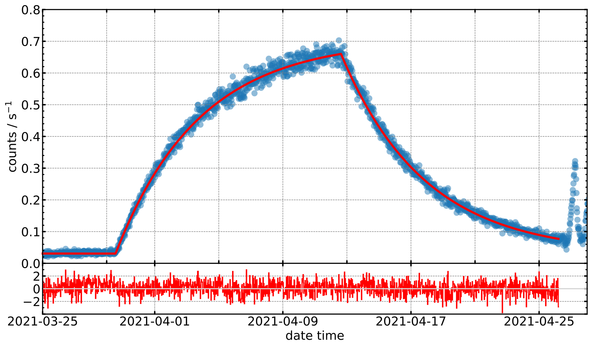
Figure 8Comparison of measured and calculated count rate in the PTB climate chamber based on a well characterized radon emanation source. Emanation source no. 2018–1121: A(Ra-226) = (1136±5) Bq produces an equilibrium activity concentration of (18.09±0.17) Bq m−3 in the climate chamber of PTB.
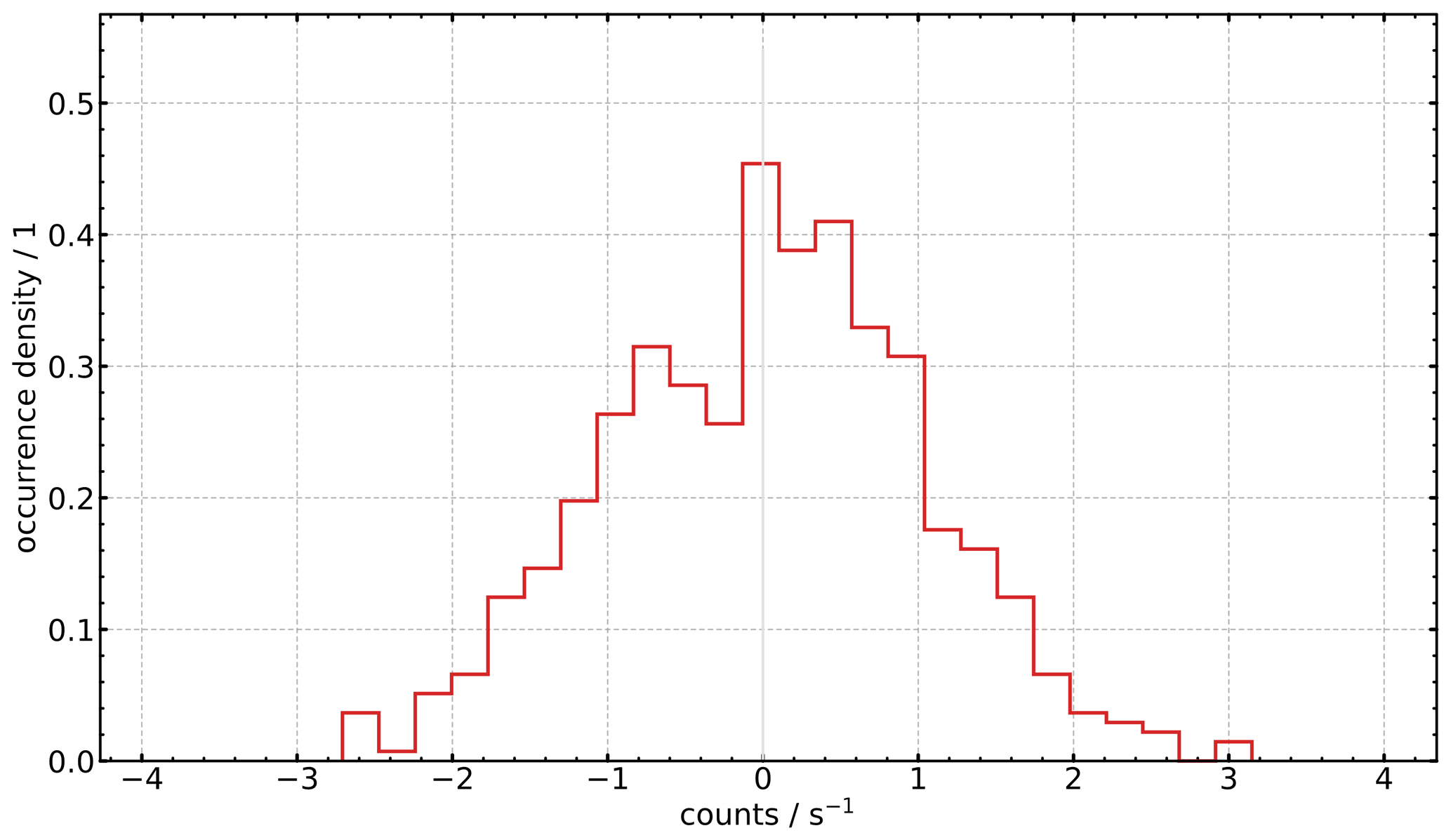
Figure 9Relative deviation between measured count rate of the reference monitor and calculated count rate from the emanation source 2018–1121 at 30 min temporal resolution shown as a histogram. The natural behaviour proves the correctness of the model, while the narrow width stresses the good statistics (low noise) of the detector even at these low activity concentrations (below 20 Bq m−3).
The PTB climate chamber tests resulted in a background estimate of (0.03107±0.00015) s−1, and a calibration factor (detector sensitivity) of (0.038460±0.0013) s−1 (Bq m−3)−1. By comparison, the background and calibration determined at ANSTO before shipping the reference monitor to PTB were 0.0178 s−1 and 0.0384 s−1 (Bq m−3)−1, respectively. As previously mentioned, the background estimate at ANSTO did not account for self-generation of radon inside the detector. It should be noted, however, that for the reference monitor calibration at ANSTO a second radon detector operating in parallel was used to estimate the ambient radon concentration at the time of peak count rate, rather than assuming a linear change in ambient radon over the calibration period, which improved the accuracy of the calibration.
3.1 A key radon dataset requiring correction/harmonization
One year of observations (meteorology, air quality and radon), starting in April 2019, were made at the Liverpool Girl's High School (LGHS), around 25 km west of Sydney, Australia. The school is situated between three arterial roads (A22, A28 and A34). The aim, of what will be a separate study, is to investigate the diurnal, synoptic and seasonal variability in public exposure to traffic-related emissions using radon as a tracer of mixing and transport processes, as demonstrated by Williams et al. (2016). While strong similarities are evident between the diurnal behaviour of the passive tracer radon and traffic-related emissions due to advection and vertical mixing (Figs. 10 and 11), some weeks after completing the campaign a problem was identified with the calibration of the 1500 L two-filter dual flow-loop radon detector employed for this study. Unless corrected, this error could significantly impact the findings of the intended study, as well as prevent the subsequent combination of this data with other radon observations in the Sydney Basin region (at Lucas Heights, Lidcombe, and Richmond) for regional modelling studies. This presented an opportunity to investigate the feasibility of transferring a calibration from the reference monitor (calibrated at PTB) to a different model radon monitor under field conditions.

Figure 10A 1-month example of hourly observations of (a) wind speed, (b) radon, (c) CO and (d) NO, on campus at the Liverpool Girl's High School for May 2019 (Chambers et al., 2022).
Radon detector calibrations for the LGHS campaign were conducted on the sampling flow (see Sect. 2.4), and background checks were performed according to method 2 (Sect. 2.3), which does not consider radon ingrowth. Since the detector was installed on a high school campus, safety regulations prevented the calibration unit (containing the 226Ra source) being setup permanently on site for automatic calibrations. Consequently, a makeshift calibration unit was brought to site every 3 months, placed on the ground, and covered from view of the students for the duration of the 6 h injection period. A summary of the resulting calibration peaks is provided in Fig. 12a.
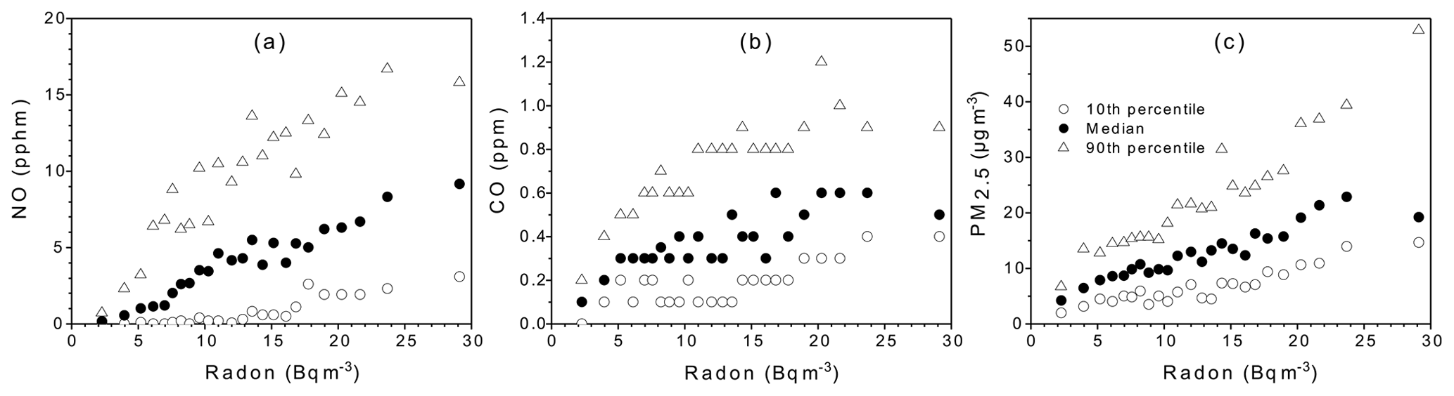
Figure 11Correlation of bin-mean radon concentration with distributions (10th, 50th, 90th) of (a) NO, (b) CO and (c) PM2.5, in Autumn (March–May) 2019, between the hours of 18:00 and 08:00 AEST (Australian Eastern Standard Time, UTC+10) each day, for predominantly stable nocturnal conditions (see Chambers et al., 2019a, for details of stability classification method). Each bin (except the last) contained 50 hourly samples.
Usually, radon concentrations in the detector reach a near constant value after ∼4 h of radon injection. An example of this behaviour for a 1500 L detector operating at Baring Head (New Zealand) is shown in Fig. 12b (red curve). Since different magnitude sources were used to calibrate the LGHS and Baring Head radon detectors, the Bearing Head calibration curve in Fig. 12b was scaled to match the initial radon build-up of the mean calibration injection for the LGHS detector.
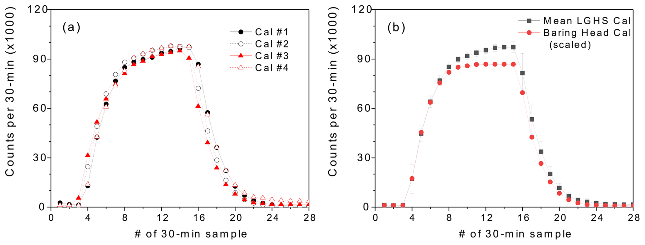
Figure 12(a) Summary of 4 calibration events for the 1500 L radon monitor, and (b) comparison of the mean LGHS calibration event with a scaled calibration event of matching duration for a 1500 L radon detector operating at a coastal site in New Zealand.
Rather than reaching a near-constant value after 4 h, the LGHS calibration curves indicated that radon concentrations continued to rise. The LGHS calibration unit had been placed on the ground, such that the ambient air inlet to flush the calibration source was only ∼5 cm from the ground. Furthermore, the unit was covered while operating, essentially forming a radon accumulation chamber from which air was being drawn to flush the source. Consequently, the calibration factor derived for the LGHS detector was too large, but by an unknown amount (see variability in Fig. 12a). After 5.5 h of injection, the ratio of net peak counts of the scaled Baring Head calibration curve to the mean LHSG calibration curve (Fig. 12b) was 0.8923.
3.2 Field comparison of reference and 1500 L radon monitors
The reference and LGHS radon monitors were setup in an air-conditioned workshop in which the temperature was maintained at (26.5±0.05) ∘C. The monitors were operated in parallel for 2 weeks, both sampling ambient outdoor air 3 m above ground level (a.g.l.) from inlets separated by several metres. Sampling was conducted on eastern side of a 3-storey building at ANSTO (−34.0526∘ N, 150.9857∘ E). It should be noted that the combination of building wake turbulence and inlet separation may contribute to small short-term differences in observed radon concentrations between the instruments under poorly mixed nocturnal conditions. Calibrated radon concentrations for both detectors are shown separately and combined in Fig. 13.
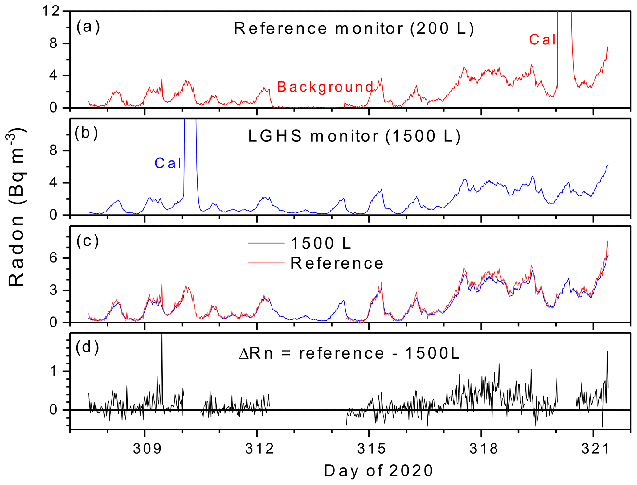
Figure 1330 min time series of calibrated radon concentrations from (a) the reference, and (b) the 1500 L monitors. All valid observations are directly compared in (c) and (d) shows the difference in radon concentration between the reference and 1500 L monitors (Chambers et al., 2022).
Bearing in mind the low radon concentrations over the comparison period (predominantly between 0.2 and 5 Bq m−3), Fig. 13c indicates that both instruments tracked relative changes in radon concentration quite reliably. The average absolute difference between the referece and 1500 L monitors (ΔRn= RnREF − Rn1500) was 0.22 Bq m−3 (Fig. 13d). Comparing Fig. 13c and d, ΔRn appears correlated with the absolute radon concentration (e.g., days 317–320), likely attributable to the suspected calibration problem with of the LGHS radon monitor.
A closer inspection of comparative detector output (Fig. 14a) indicates at least two other factors contributing to ΔRn: (i) a higher counting uncertainty of the reference monitor (sample to sample variability) due to its smaller delay chamber, and (ii) a faster response time of the reference monitor.
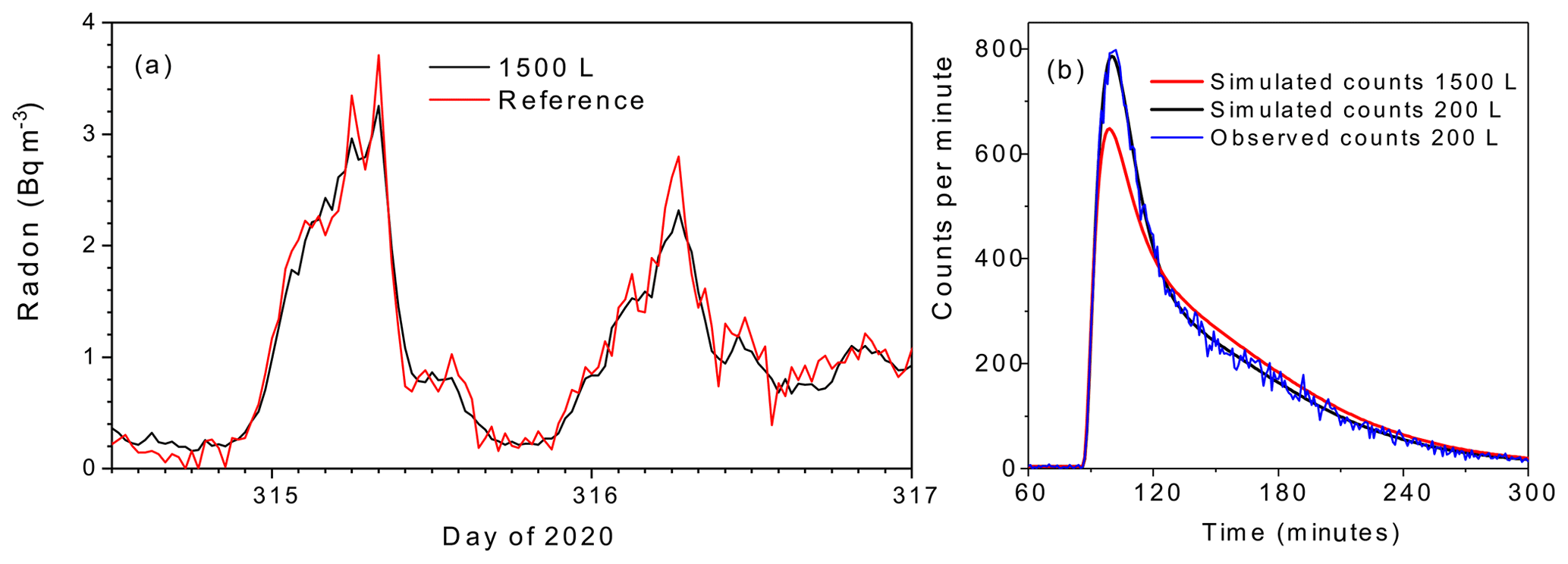
Figure 14(a) Expanded view of direct comparison between the reference and 1500 L monitors at 30 min temporal resolution, and (b) normalised simulated response of the reference and 1500 L monitors to a 1 min radon injection.
Ideally, two-filter radon detector results should be response time corrected prior to interpretation according to Griffiths et al. (2016). However, a problem with the configuration of the thoron delay volume of the reference monitor, which was only diagnosed and rectified after this comparison was performed, prevented these corrections from being made. COVID-19 restrictions delayed the repair of the thoron delay and prevented the intercomparison being repeated prior to the submission deadline for this study.
Numerical models were devised for both monitors (as per Griffiths et al., 2016), assuming optimal configuration of both detectors and delay volumes, and used to simulate their respective response to a radon pulse. As evident from the normalised simulated count rate in Fig. 14b, the reference monitor responds more rapidly than the 1500 L model to a 1 min radon spike. This faster response time leads to an increase in amplitude of relatively quick changes in ambient radon concentration.
Regressing the output of the 1500 L and reference monitors (Fig. 15a) indicates only a small calibration offset (A0=0.0505 Bq m−3) but a substantial underestimate of the calibration gain (A1=0.8917), the value of which closely matched the ratio of calibration peaks (0.8923; Sect. 3.1, Fig. 12b). Concentration ratios (; Fig. 15b) were largest below radon concentrations of ∼0.3 Bq m−3, which is approaching the detection limit of the reference monitor. It should also be noted that ratios are poorly defined between very small values.

Figure 15(a) regression of 1500 L and reference monitor radon observations, and (b) dependence of the L ratio on absolute radon concentration as measured by the reference monitor.
3.3 Transferring the reference monitor calibration to the 1500 L detector
The offset of 50.5 mBq m−3 between the 1500 L and reference monitor (Fig. 15a) corresponds to an background contribution of ∼0.85 min−1, which was ∼34 % of the estimated 1500 L monitor background of (2.5±0.37) min−1. This is reasonably consistent with the PTB background tests which indicated that the contribution of self-generated radon within a detector may contribute a significant fraction of the overall background count. However, the uncertainty in the 1500 L monitor background estimate (i.e., σ±0.37 min−1) would also be a contributing factor. The background contribution arising from radon ingrowth is expected to vary randomly from one detector to the next (arising from batch to batch variability in trace 226Ra contamination of construction materials). Historically this contribution has been neglected for the larger model (1500 and 700 L) two-filter monitors since it was not readily quantifiable. However, it appears that this can be rectified when transferring a traceable calibration from a reference monitor.
The more significant discrepancy between the two monitors is indicated by the regression slope, A1=0.8917 (Fig. 15a). Considering the high R2 value (0.98), and similarity of the slope to the estimated calibration error in Sect. 3.1, it is likely the discrepancy is entirely attributable to the incorrect calibration of the LGHS 1500 L monitor. Fortunately, it appears that even this short (2-week) field intercomparison is sufficient to transfer a calibration from the reference monitor to a larger model similar detector, to correct the problematic calibration, and harmonize radon observations with other observations in the Sydney Basin region.
Based on Fig. 15a, the output of the LGHS radon monitor was scaled by and an offset of −0.0505 Bq m−3 was applied. Results of the subsequent regression between the reference monitor and corrected LGHS output are presented in Fig. 16a, which indicates a successful transfer of the calibration from the reference monitor.
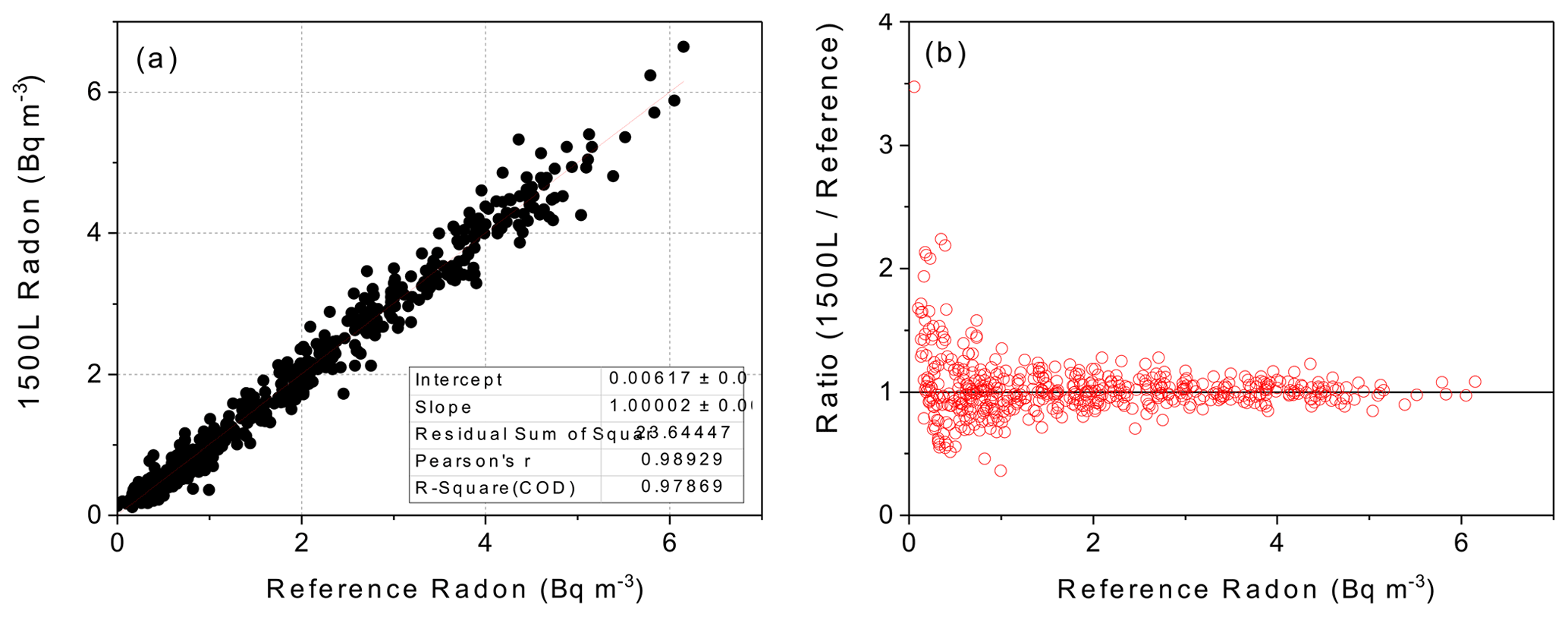
Figure 16(a) regression of corrected 1500 L radon monitor observations with reference monitor observations, and (b) ratio of corrected to reference observations as a function of ambient radon concentration.
The majority of high values for the LGHS to reference monitor ratio (Fig. 16b) occurred during the day, when mixing was strongest and ambient radon concentrations lowest (Fig. 17a). This suggests that the larger counting uncertainty and faster response time of the reference monitor likely contribute more to the R2<1 in Fig. 16a than the separation between the detector inlets for the duration of the intercomparison. Following the calibration transfer, differences between the two instruments (which had not been response time corrected) were distributed more evenly about zero, with an absolute magnitude typically <0.5 Bq m−3 (Fig. 17b). This is unsurprising given the difference in estimated DLs for the two monitors, 0.2 and 0.025 Bq m−3, for the reference and LGHS monitors, respectively.

Figure 17(a) Median and 90th percentile values of the LGHS to reference monitor ratio over a composite diurnal cycle formed from the whole 2-week measurement period, and (b) corrected and uncorrected concentration differences between the montors.
The primary advantages of the new reference monitor are its portability and low flow rate, which enable (i) traceable calibration under laboratory conditions, (ii) more accurate field calibrations, and (iii) simpler comparison with, and calibration transfer to, existing radon monitors. This capability will enhance efforts to harmonise radon measurements across European monitoring networks, a key goal of the 19ENV01 traceRadon Project. The main disadvantage is the higher DL (∼0.14 Bq m−3) compared to larger model detectors (0.025 Bq m−3). However, this would not impact observations at most inland sites.
The vertical orientation and secure mounting of the reference monitor's measurement head enables transport without the need to remove the head. This improves calibration stability, simplifies operation, and improves monitor suitability for use on mobile platforms (provided the DL is fit for purpose). Based on the gradual, but approximately linear, changes in sensitivity and background of two-filter radon monitors, the reference monitor's calibration should be checked in a climate chamber over a 4 to 6-week period at least every two years, to verify (or “nudge”) the field calibrations.
Here we demonstrated that a 2-week comparison period is sufficient to transfer a calibration to a similar instrument. When transferring a calibration to a monitor operating by a different measurement principle, however, a longer comparison period (≥1 month) would be prudent, to cover a broader range of meteorological conditions.
The reference monitor used in this study was a prototype, for which the empirical DL was ∼0.2 Bq m−3. After correcting the plumbing of the thoron delay, and optimising the speed of the internal flow loop, the theoretical DL of ∼0.14 Bq m−3 should be achievable. To be suitable for remote “baseline” studies a radon monitor requires a DL of ≤50 mBq m−3 (Zahorowski et al., 2013; Chambers et al., 2016). The best opportunity to improve the DL of this monitor is through improving the counting efficiency of the measurement head (Fig. 1b). Based on the detector model presented by Griffiths et al. (2016), a more efficient head design has the potential to increase counting efficiency by a factor of 3–4. If realised, this will greatly increase the range of research applications for the new portable radon monitor.
We introduce and describe a prototype 200 L two-filter dual flow-loop 222Rn monitor for which a calibration traceable to the SI has been established for the first time. Portable monitors of this kind can make direct radon measurements at 30 min temporal resolution with a detection limit (defined as the radon concentration at which the counting error reaches 30 %) of ∼0.14 Bq m−3. We summarise the first field trials of this monitor and use the results to demonstrate its suitability for use as a calibration transfer device for existing radon detectors in global monitoring networks to harmonise their output. In conjunction with improved radon flux maps (Röttger et al., 2021; Levin et al., 2021), this capability has the potential to reduce uncertainty in local- to regional-scale greenhouse gas emissions estimates presently being made using the Radon Tracer Method. The compact nature of this monitor, compared with existing models of two-filter detectors, makes high quality, high temporal resolution radon concentration measurements accessible for a much broader range of sites where space and power restrictions have previously presented an obstacle. With anticipated advancements in measurement head design, this portable instrument will achieve a detection limit suitable for even remote “baseline” monitoring.
The main datasets underpinning the results and discussion of this manuscript are available directly from the corresponding author, in the Supplement, or online from https://doi.org/10.13140/RG.2.2.20639.02725 (Chambers et al., 2022).
The supplement related to this article is available online at: https://doi.org/10.5194/adgeo-57-63-2022-supplement.
Scoping and planning of the manuscript was performed by SDC, SR, ADG, and AGW. Construction, testing and modification of the 200 and 1500 L radon detectors was undertaken by OS and VM. The planning and execution of field work was undertaken by OS, SDC, and ADG. Calibration of instruments in the field was performed by OS, ADG, and SDC. The use of SI traceable sources to develop the traceable laboratory calibration of the 200 L detector was performed by SR, FM, AR, and VM. Software development was undertaken by ADG. Data analysis was performed by SDC and SR. Drafting of the initial manuscript and preparation of all figures was performed by SDC and SR. Project administration and funding was arranged by AR and AGW. All authors contributed to the checking, editing and revision of the manuscript at each stage.
The contact author has declared that neither they nor their co-authors have any competing interests.
Publisher's note: Copernicus Publications remains neutral with regard to jurisdictional claims in published maps and institutional affiliations.
This article is part of the special issue “Geoscience applications of environmental radioactivity (EGU21 GI6.2 session)”. It is a result of the EGU General Assembly 2021, 19–30 April 2021.
The authors would like to acknowledge the efforts of retired technician Sylvester Werczynski for development of early versions of the radon monitor software.
This research has been supported by the European Metrology Programme for Innovation and Research (grant no. 19ENV01 traceRadon).
This paper was edited by Anita Erőss and reviewed by Istvan Csige and one anonymous referee.
Balkanski, Y. J., Jacob, D. J., Arimoto, R., and Kritz, M. A.: Distribution of 222Rn over the North Pacific: Implications for continental influences, J. Atmos. Chem., 14, 353–374, 1992.
Basic Safety Standards Directive (BSSD): Official Journal of the European Union, L 13. Legislation, English Edition, https://eur-lex.europa.eu/legal-content/EN/TXT/PDF/?uri=OJ:L:2014:013:FULL&from=EN (last access: 10 May 2022), vol. 57, 17 January 2014, ISSN 1977-0677, 2013.
Biraud, S.: Vers la régionalisation des puits et sources des composes à effet de serre: analyse de la variabilité synoptique à l'observatoire de Mace Head, Irlande, PhD Thesis, University of Paris VII, France, 2000.
Chambers, S. D., Williams, A. G., Zahorowski, W., Griffiths, A. D., and Crawford, J.: Separating remote fetch and local mixing influences on vertical radon measurements in the lower atmosphere, Tellus B, 17, 843–859, https://doi.org/10.1111/j.1600-0889.2011.00565.x, 2011.
Chambers, S. D., Hong, S.-B., Williams, A. G., Crawford, J., Griffiths, A. D., and Park, S.-J.: Characterising terrestrial influences on Antarctic air masses using Radon-222 measurements at King George Island, Atmos. Chem. Phys., 14, 9903–9916, https://doi.org/10.5194/acp-14-9903-2014, 2014.
Chambers, S. D., Williams, A. G., Conen, F., Griffiths, A. D., Reimann, S., Steinbacher, M., Krummel, P. B., Steele, L. P., van der Schoot, M. V., Galbally, I. E., Molloy, S. B., and Barnes, J. E.: Towards a universal “baseline” characterisation of air masses for high- and low-altitude observing stations using Radon-222, Aerosol Air Qual. Res., 16, 885–899, https://doi.org/10.4209/aaqr.2015.06.0391, 2016.
Chambers, S. D., Preunkert, S., Weller, R., Hong, S.-B., Humphries, R. S., Tositti, L., Angot, H., Legrand, M., Williams, A. G., Griffiths, A. D., Crawford, J., Simmons, J., Choi, T. J., Krummel, P. B., Molloy, S., Loh, Z., Galbally, I., Wilson, S., Magand, O., Sprovieri, F., Pirrone, N., and Dommergue, A.: Characterizing Atmospheric Transport Pathways to Antarctica and the Remote Southern Ocean Using Radon-222, Front. Earth Sci., 6, 1–28, https://doi.org/10.3389/feart.2018.00190, 2018.
Chambers, S. D., Guérette, E.-A., Monk, K., Griffiths, A. D., Zhang, Y., Duc, H., Cope, M., Emmerson, K. M., Chang, L. T., Silver, J. D., Utembe, S., Crawford, J., Williams, A. G., and Keywood, M.: Skill-testing chemical transport models across contrasting atmospheric mixing states using Radon-222, Atmosphere, 10, 25, https://doi.org/10.3390/atmos10010025, 2019a.
Chambers, S. D., Podstawczyńska, A., Pawlak, W., Fortuniak, K., Williams, A. G., and Griffiths, A. D.: Characterising the state of the urban surface layer using Radon-222, J. Geophys. Res.-Atmos., 124, 770–788, https://doi.org/10.1029/2018JD029507, 2019b.
Chambers, S., Morosh, V., Griffiths, A., Williams, A., Röttger, S., and Röttger, A.: Field testing of a portable two-filter dual-flow-loop 222Rn detector, EGU General Assembly 2021, online, 19–30 Apr 2021, EGU21-196, https://doi.org/10.5194/egusphere-egu21-196, 2021.
Chambers, S., Griffiths, A., Williams, A., Sisoutham, O., Morosh, V., Röttger, S., Mertes, F., and Röttger, A.: Source data for “Portable two-filter dual-flow-loop 222Rn detector: stand-alone monitor and calibration transfer device” in Advances in Geoscience, ResearchGate [data set], https://doi.org/10.13140/RG.2.2.20639.02725, 2022.
Choi, E., Komori, M., Takahisa, K., Kudomi, N., Kume, K., Hayashi, K., Yoshida, S., Ohsumi, H., Ejiri, H., Kishimoto, T., Matsuoka, K., and Tasaka, S.: Highly sensitive radon monitor and radon emanation rates for detector components, Nuclear Instruments and Methods in Physics Research A, 459, 177–181, 2001.
Curcoll Masanes, R., Grossi, C., and Vargas, A.: High efficiency and portable monitor of atmospheric radon concentration activity for environmental applications, EGU General Assembly 2021, online, 19–30 April 2021, EGU21-4497, https://doi.org/10.5194/egusphere-egu21-4497, 2021.
Fontan, J., Guedalia, D., Druilhet, A., and Lopez, A.: Une method de mesure de la stabilite verticale de l'atmosphere pres du sol, Bound.-Lay. Meteorol., 17, 3–14, https://doi.org/10.1007/BF00121933, 1979.
Fujinami, N. and Osaka, S.: Variations in radon 222 daughter concentrations in surface air with atmospheric stability, J. Geophys. Res., 92, 1041–1043, 1987.
Griffiths, A. D., Chambers, S. D., Williams, A. G., and Werczynski, S.: Increasing the accuracy and temporal resolution of two-filter radon–222 measurements by correcting for the instrument response, Atmos. Meas. Tech., 9, 2689–2707, https://doi.org/10.5194/amt-9-2689-2016, 2016.
Grossi, C., Arnold, D., Adame, A. J., Lopez-Coto, I., Bolivar, J. P., de la Morena, B. A., and Vargas, A.: Atmospheric 222Rn concentration and source term at El Arenosillo 100 m meteorological tower in southwest Spain, Radiat. Meas., 47, 149–162, https://doi.org/10.1016/j.radmeas.2011.11.006, 2012.
Grossi, C., Vogel, F. R., Curcoll, R., Àgueda, A., Vargas, A., Rodó, X., and Morguí, J.-A.: Study of the daily and seasonal atmospheric CH4 mixing ratio variability in a rural Spanish region using 222Rn tracer, Atmos. Chem. Phys., 18, 5847–5860, https://doi.org/10.5194/acp-18-5847-2018, 2018.
Grossi, C., Chambers, S. D., Llido, O., Vogel, F. R., Kazan, V., Capuana, A., Werczynski, S., Curcoll, R., Delmotte, M., Vargas, A., Morguí, J.-A., Levin, I., and Ramonet, M.: Intercomparison study of atmospheric 222Rn and 222Rn progeny monitors, Atmos. Meas. Tech., 13, 2241–2255, https://doi.org/10.5194/amt-13-2241-2020, 2020.
Hosler, C. R.: Urban–rural climatology of atmospheric radon concentrations, J. Geophys. Res., 73, 1155–1166, 1968.
IAEA SSS: Protection of the Public against Exposure Indoors due to Radon and Other Natural Sources of Radiation, Safety Standards Series No. SSG-32, STI/PUB/1651 978-92-0-102514-2, 90 pp., 2015.
Jacobi, W.: The history of the radon problem in mines and homes, Annals of the ICRP, https://doi.org/10.1016/0146-6453(93)90012-W, 1993.
Jacobi, W. and André, K.: The vertical distribution of Radon 222, Radon 220 and their decay products in the atmosphere, J. Geophys. Res., 68, 3799–3814, 1963.
Kikaj, D., Chambers, S. D., Kobal, M., Crawford, J., and Vaupotic, J.: Characterising atmospheric controls on winter urban pollution in a topographic basin setting using Radon-222, Atmos. Res., 237, 104838, https://doi.org/10.1016/j.atmosres.2019.104838, 2020.
Kirichenko, L. V.: Radon exhalation from vast areas according to vertical distributions of its short-lived decay products, J. Geophys. Res., 75, 3639–3649, 1970.
Kritz, M. A., Rosner, S. W., and Stockwell, D. Z.: Validation of an off-line three-dimensional chemical transport model using observed radon profiles: 1 Observations, J. Geophys. Res., 103, 8425–8432, https://doi.org/10.1029/97JD02655, 1998.
Levin, I., Glatzel-Mattheier, H., Marik, T., Cuntz, M., Schmidt, M., and Worthy, D. E.: Verification of German methane emission inventories and their recent changes based on atmospheric observations, J. Geophys. Res., 104, 3447–3456, 1999.
Levin, I., Born, M., Cuntz, M., Langendörfer, U., Mantsch, S., Naegler, T., Schmidt, M., Varlagin, A., Verclas, S., and Wagenbach, D.: Observations of atmospheric variability and soil exhalation rate of radon-222 at a Russian forest site – Technical approach and deployment for boundary layer studies, Tellus B, 54, 462–475, https://doi.org/10.1034/j.1600-0889.2002.01346.x, 2002.
Levin, I., Schmithüsen, D., and Vermeulen, A.: Assessment of 222radon progeny loss in long tubing based on static filter measurements in the laboratory and in the field, Atmos. Meas. Tech., 10, 1313–1321, https://doi.org/10.5194/amt-10-1313-2017, 2017.
Levin, I., Gachkivskyi, M., Maurer, L., Della Coletta, J., Karstens, U., Chambers, S. D., and Griffiths, A. D.: Development of Heidelberg Radon Monitor (HRM) data evaluation for ICOS and update of HRM – ANSTO comparisons at the Karlsruhe (KIT) tall tower station, ICOS Science Conference 2020, 15–17 September, Utrecht, the Netherlands, 2020.
Levin, I., Karstens, U., Hammer, S., DellaColetta, J., Maier, F., and Gachkivskyi, M.: Limitations of the radon tracer method (RTM) to estimate regional greenhouse gas (GHG) emissions – a case study for methane in Heidelberg, Atmos. Chem. Phys., 21, 17907–17926, https://doi.org/10.5194/acp-21-17907-2021, 2021.
Liu, S. C., McAfee, J. R., and Cicerone, R. J.: Radon 222 and tropospheric vertical transport, J. Geophys. Res., 89, 7291–7297, https://doi.org/10.1029/JD089iD05p07291, 1984.
Locatelli, R., Bousquet, P., Hourdin, F., Saunois, M., Cozic, A., Couvreux, F., Grandpeix, J.-Y., Lefebvre, M.-P., Rio, C., Bergamaschi, P., Chambers, S. D., Karstens, U., Kazan, V., van der Laan, S., Meijer, H. A. J., Moncrieff, J., Ramonet, M., Scheeren, H. A., Schlosser, C., Schmidt, M., Vermeulen, A., and Williams, A. G.: Atmospheric transport and chemistry of trace gases in LMDz5B: evaluation and implications for inverse modelling, Geosci. Model Dev., 8, 129–150, https://doi.org/10.5194/gmd-8-129-2015, 2015.
Melintescu, A., Chambers, S. D., Crawford, J., Williams, A. G., Zorila, B., and Galeriu, D.: Radon-222 related influence on ambient gamma dose, J. Env. Rad., 189, 67–78, https://doi.org/10.1016/j.jenvrad.2018.03.012, 2018.
Mertes, F., Röttger, S., and Röttger, A.: Approximate sequential Bayesian filtering to estimate Rn-222 emanation from Ra-226 sources from spectra, SMSI, https://doi.org/10.5162/SMSI2021/D3.3, 2021.
Mertes, F., Kneip, N., Heinke, R., Kieck, T., Studer, D., Weber, F., Röttger, S., Röttger, A., Wendt, K., and Walther, C.: Ion implantation of 226Ra for a primary 222Rn emanation standard, Appl. Radiat. and Isotopes, 181, 110093, https://doi.org/10.1016/j.apradiso.2021.110093, 2022a.
Mertes, F., Röttger, S., Röttger, A.: Development of 222Rn emanation sources with integrated quasi 2 active monitoring, Int. J. Environ. Res. Pub. He., 19, 840, https://doi.org/10.3390/ijerph19020840, 2022b.
Moses, H., Stehney, A. F., and Lucas, H. F. J.: The effect of meteorological variables upon the vertical and temporal distributions of atmospheric radon, J. Geophys. Res., 65, 1223–1238, 1960.
Pereira, E. B.: Time series measurements in the Antarctic Peninsula (1986–1987), Tellus, 42B, 39–45, 1990.
Perrino, C., Pietrodangelo, A., and Febo, A.: An atmospheric stability index based on radon progeny measurements for the evaluation of primary urban pollution, Atmos. Environ., 35, 5235–5244, 2001.
Polian, G.: Les transports atmosphériques dans l'hémisphère sud et le bilan global du radon-222, PhD Thesis, University of Paris VI, France, 1986.
Polian, G., Lambert, G., Ardouin, B., and Jegou, A.: Long-range transport of continental radon in subantarctic and Antarctic areas, Tellus B, 38, 178–189, 1996.
Porstendörfer, J.: Properties and behaviour of Radon and Thoron and their decay products in the air, J. Aerosol Sci., 25, 219–263, 1994.
Porstendörfer, J., Pagelkopf, P., and Gründel, M.: Fraction of the positive 218Po and 214Pb clusters in indoor air, Radiat. Prot. Dosimetry, 113, 342–351, https://doi.org/10.1093/rpd/nch465, 2005.
Röttger, A., Röttger, S., Grossi, C., Vargas, A., Curcoll, R., Otáhal, P., Hernández-Ceballos, M. A., Cinelli, G., Chambers, S. D., Barbosa, S. A., Ioan, M.-A., Radulescu, I., Kikaj, D., Chung, E., Arnold, T., Yver-Kwok, C., Fuente, M., Mertes, F., and Morosh, V.: New metrology for radon at the environmental level, Meas. Sci. Technol., 32, 124008, https://doi.org/10.1088/1361-6501/ac298d, 2021.
Satterly, J.: On the Amount of Radium Emanation in the Lower Regions of the Atmosphere and Its Variation with the Weather, Philos. Mag., 20, 1–36, 1910.
Schery, S. D., Gaeddert, D. H., and Wilkening, H. M.: Two-filter monitor for atmospheric 222Rn, Rev. Sci. Instrum., 51, 338–343, https://doi.org/10.1063/1.1136214, 1980.
Schmithüsen, D., Chambers, S., Fischer, B., Gilge, S., Hatakka, J., Kazan, V., Neubert, R., Paatero, J., Ramonet, M., Schlosser, C., Schmid, S., Vermeulen, A., and Levin, I.: A European-wide 222radon and 222radon progeny comparison study, Atmos. Meas. Tech., 10, 1299–1312, https://doi.org/10.5194/amt-10-1299-2017, 2017.
Sesana, L., Caprioli, E., and Marcazzan, G. M.: Long period study of outdoor radon concentration in Milan and correlation between its temporal variations and dispersion properties of atmosphere, J. Environ. Radioact., 65, 147–160, https://doi.org/10.1016/S0265-931X(02)00093-0, 2003.
Thomas, J. W. and LeClare, P. C.: A study of the two-filter method for radon-222, Health Phys., 18, 113–124, 1970.
Tositti, L., Pereira, E. B., Sandrini, S., Capra, D., Tubertini, O., and Bettoli, M. G.: Assessment of summer trends of tropospheric radon isotopes in a costal Antarctic station (Terra Nova Bay), Int. J. Environ. An. Ch., 82, 259–274, 2002.
Vargas, A., Arnold, D., Adame, J. A., Grossi, C., Hernández-Ceballos, M. A., and Bolívar, J. P.: Analysis of the vertical radon structure at the Spanish “El Arenosillo” tower station, J. Environ. Radioactiv., 139, 1–17, https://doi.org/10.1016/j.jenvrad.2014.09.018, 2015.
Wada, A., Murayama, S., Kondo, H., Matsueda, H., Sawa, Y., and Tsuboi, K.: Development of a compact and sensitive electrostatic radon-222 measuring system for use in atmospheric observation, J. Meteorol. Soc. Jpn. Ser. II, 88, 123–134, https://doi.org/10.2151/jmsj.2010-202, 2010.
Wada, A., Matsueda, H., Murayama, S., Taguchi, S., Kamada, A., Nosaka, M., Tsuboi, K., and Sawa, Y.: Evaluation of anthropogenic emissions of carbon monoxide in East Asia derived from the observations of atmospheric radon-222 over the western North Pacific, Atmos. Chem. Phys., 12, 12119–12132, https://doi.org/10.5194/acp-12-12119-2012, 2012.
Whittlestone, S.: A high sensitivity Rn detector incorporating a particle generator, Health Phys., 49, 847–852, 1985.
Whittlestone, S. and Zahorowski, W.: Baseline radon detectors for shipboard use: development and deployment in the First Aerosol Characterization Experiment (ACE 1), J. Geophys. Res., 103, 16743–16751, https://doi.org/10.1029/98JD00687, 1998.
WHO: Handbook on Indoor Radon: A Public Health Perspective, Geneva, WHO, 2009.
Williams, A. G. and Chambers, S. D.: A history of radon measurements at Cape Grim, Baseline Atmospheric Program (Australia) History and Recollections (40th Anniversary Special Edition), 131–146, 2016.
Williams, A. G., Zahorowski, W., Chambers, S. D., and Griffiths, A.: The vertical distribution of radon in clear and cloudy daytime terrestrial boundary layers, J. Atmos. Sci., 68, 155–174, https://doi.org/10.1175/2010JAS3576.1, 2011.
Williams, A. G., Chambers, S. D., and Griffiths, A. D.: Bulk mixing and decoupling of the nocturnal stable boundary layer characterized using a ubiquitous natural tracer, Bound.-Lay. Meteorol., 20, 381–402, https://doi.org/10.1007/s10546-013-9849-3, 2013.
Wright, J. R. and Smith, O. F.: The Variation with Meteorological Conditions of the Amount of Radium Emanation in the Atmosphere, in the Soil Gas, and in the Air Exhaled from the Surface of the Ground, at Manila, Phys. Rev., 5, 459–482, 1915.
Zahorowski, W., Griffiths, A. D., Chambers, S., Williams, A. G., Law, R. M., Crawford, J., and Werczynski, S.: Constraining annual and seasonal radon-222 flux density from the Southern Ocean using radon-222 concentrations in the boundary layer at Cape Grim, Tellus B, 65, 19622, https://doi.org/10.3402/tellusb.v65i0.19622, 2013.
Zhang, B., Liu, H., Crawford, J. H., Chen, G., Fairlie, T. D., Chambers, S., Kang, C.-H., Williams, A. G., Zhang, K., Considine, D. B., Sulprizio, M. P., and Yantosca, R. M.: Simulation of radon-222 with the GEOS-Chem global model: emissions, seasonality, and convective transport, Atmos. Chem. Phys., 21, 1861–1887, https://doi.org/10.5194/acp-21-1861-2021, 2021.
Zhang, K., Wan, H., Zhang, M., and Wang, B.: Evaluation of the atmospheric transport in a GCM using radon measurements: sensitivity to cumulus convection parameterization, Atmos. Chem. Phys., 8, 2811–2832, https://doi.org/10.5194/acp-8-2811-2008, 2008.