 | 26 May 2023
Forecasting changes of the flow regime at deep geothermal wells based on high resolution sensor data and low resolution chemical analyses
Annette Dietmaier
Geothermal waters provide a great resource to generate clean energy, however, there is a notorious lack of high quality data on these waters. The scarcity of deep geothermal aquifer information is largely due to inaccessibility and high analysis costs. However, multiple operators use geothermal wells in Lower Bavaria and Upper Austria for balneological (medical and wellness) applications as well as for heat mining purposes. The state of the art sampling strategy budgets for a sampling frequency of 1 year. Previous studies have shown that robust groundwater data requires sampling intervals of 1–3 months, however, these studies are based on shallow aquifers which are more likely to be influenced by seasonal changes in meteorological conditions. This study set out to assess whether yearly sampling adequately represents sub-yearly hydrochemical fluctuations in the aquifer by comparing yearly with quasi-continuous hydrochemical data at two wells in southeast Germany by assessing mean, trend and seasonality detection among the high and low temporal resolution data sets. Furthermore, the ability to produce reliable forecasts based on yearly data was examined. In order to test the applicability of virtual sensors to elevate the information content of yearly data, correlations between the individual parameters were assessed. The results of this study show that seasonal hydrochemical variations take place in deep aquifers, and are not adequately represented by yearly data points, as they are typically gathered at similar production states of the well and do not show varying states throughout the year. Forecasting on the basis of yearly data does not represent the data range of currently measured continuous data. The limited data availability did not allow for strong correlations to be determined. We found that annual measurements, if taken at regular intervals and roughly the same production rates, represent only a snapshot of the possible hydrochemical compositions. Neither mean values, trends nor seasonality was accurately captured by yearly data. This could lead to a violation of stability criteria for mineral water, or to problems in the geothermal operation (scalings, degassing). We thus recommend a new testing regime of at least 3 samples a year. While not a replacement for the detailed analyses, under the right circumstances, and when trained with more substantial data sets, viertual sensors provide a robust method in this setting to trigger further actions.
- Article
(1070 KB) - Full-text XML
-
Supplement
(890 KB) - BibTeX
- EndNote


Facing an acute energy crisis and a global climate crisis, Europe must search for alternative energy sources to imported oil and gas. Deep geothermal waters can provide an important source of energy. However, there is a notorious lack of reliable data regarding these waters (Krieger et al., 2022): current exploitation of deep groundwater consists of clustered wells which are widely distributed over large areas, which limits the spatial resolution of available data points, while sampling and analysis costs (typically between EUR 1500 and more than EUR 10 000, depending on the number of parameters) limit the frequency at which hydrochemical assessments can be conducted (Alley et al., 2013; Hebig et al., 2012; Krieger et al., 2022). At meaningful sampling intervals the costs for conventional analyses are on the same order as the equipment for online-measurements. Since deep groundwater aquifers play a negligible role in daily drinking water provision, these aquifers are not as present in public interest as, e.g., shallow ground water or surface water bodies. However, even the large number of hydrochemical analyses of groundwater wells available to this study, which includes research wells, display a similar data scarcity.
Insufficient in-situ data makes numerical modelling of subsurface dynamics difficult and limits the reliability of groundwater monitoring networks (Hebig et al., 2012; Caers and Castro, 2006). Furthermore, deep groundwater acts as a safety net for times when shallow groundwater resources are depleted. Monitoring the development of its hydrochemical quality is thus of utmost importance (Kang et al., 2019) and one of the main purposes of the European Water Framework Directive (WFD) (European Parliament and Council, 2000). This study focuses on a deep geothermal groundwater body exploited for heat and energy production and medical spas. In this setting, hydrochemical and geophysical information serves as an indicator of the geographical course of the groundwater's flow paths. It further helps describe processes taking place along these flow paths in the rock matrix (Birner et al., 2011; Mayrhofer et al., 2014; Heine et al., 2021). Additionally, fluctuations in the hydrochemical composition can have severe effects on the longevity of the geothermal power plant hardware (e.g. corrosion and scaling) and, in the case of medical wellness applications, on the certification as a medical thermal spa. This information is not only relevant for present conditions. Forecasts are highly valuable to well operators for long-term sustainable well exploitation strategies and are explicitly required by the WFD (European Parliament and Council, 2000).
The state of the art deep groundwater sampling procedure typically budgets for yearly physical and chemical analyses. This frequency is codified in national guidelines, such as the “Definitions and Quality Standards for Medical Wellness” in Germany (Deutscher Heilbäderverband and Deutscher Tourismusverband, 2016). However, optimal sampling frequency is not an arbitrary value, but can be defined in terms of providing as much information as possible with as few sampling points as necessary (Nelson and Ward, 1981). The term information, in turn, can be defined, in a statistical sense, in terms of the variance of the mean (Barcelona et al., 1989): Var, where x is the sample mean, σ is the variance and n is the number of samples. While information content rises with an increase of samples, given the costs, redundancies must be avoided (Barcelona et al., 1989).
In 1989, the US Environmental Protection Agency published a report on sampling frequency for groundwater quality monitoring (Barcelona et al., 1989) in which the investigators used data from a bi-weekly sampling campaign to derive optimal sampling intervals for a shallow sand and gravel aquifer in Illinois, USA. Basing their investigation on the assessment of auto-correlation and information loss at different sampling intervals, they found an optimal groundwater sampling frequency of around 2 to 3 months (Barcelona et al., 1989). In contrast, Zhou (1996) names three quantitative components (trend detection, determination of seasonal variability and estimation of mean) through which diverging sampling intervals can be compared to each other. In their case study at Spannenburg Pumping Station in the Netherlands they derive an optimal sampling interval for hydrochemical and geophysical analyses of 1 month. Financially and logistically, this might pose an impossible sampling strategy for many deep wells. If increasing sampling frequencies is not an option, elevating information through virtual sensors (VS) might be a viable alternative. VS are a software sensor layer which produces signals as indirect measurements of process variables by combining signals from physical sensors or other VS, physical laws and statistical models (Martin et al., 2021; Kabadayi et al., 2006; Porter et al., 2000). Among the advantages of VS are lower initial and ongoing costs and their ability to be deployed in hostile environments where inaccessibility limits the application of physical sensors (Tegen et al., 2019), all of which aids in optimizing maintenance and management processes (Porter et al., 2000). VS have been applied to groundwater monitoring applications before: Porter et al. (2000) used data fusion modeling to construct a groundwater flow model of a local river site. They point out that data fusion modeling solves the problem of combining point data for hydraulic head and conductivity. In order to fill months long data gaps in time series of a geothermal heating plant's energy demand, Baumann et al. (2017) used daily mean air temperatures and a typical control function for domestic boilers to calculate produced geothermal energy and derive flow rates and injection temperatures. Seasonal fluctuations and effects of sudden changes in energy demand were also represented with high accuracy.
Given the common practice of yearly hydrochemical analyses for German deep groundwater wells, which oppose the points raised in the aforementioned studies regarding optimal sampling frequency determination, the question arises whether the current sampling strategy accurately represents true fluctuations taking place in the aquifer. It is important to note that all studies conducted on this question have focused on shallow aquifers. It is thus of vital importance to asses the information content of yearly data in comparison to high frequency data gathered in a deep geothermal aquifer and explore options of elevating it through VS. In this study, we compare yearly and daily hydrochemical and physical (e.g. temperature, pressure, volume) data gathered in a deep geothermal aquifer in Bavaria, Germany, in order to answer the following questions: (i) can yearly data adequately represent mean, seasonal variability and trends of quasi-continuous data? (ii) is yearly data a sufficient base for long-term forecasting of hydrochemical compositions of deep groundwater? (iii) can virtual sensors be used to elevate information content of rudimentary data sets in this environment?
2.1 Study Area and Geology
This study uses hydrochemical samples taken at two wells in the Northern Alpine Foreland Basin (NAFB). Most waters in the Upper Jurassic Aquifer in the northern and northeastern part of the NAFB are characterized as Ca-(Mg)-HCO3 water with low salinity (<0.9 g L−1), but there are waters with total dissolved salts (TDS) values of >2 g L−1 at the edge of the helvetic facies close to hydrocarbon deposits (Birner et al., 2011; Birner, 2013). Inflow from underlying or overlying strata change the general characteristics. Waters from Dogger, Keuper and Lias carry water of the types sodium-sulfate-bicarbonate (sampled in Bad Überkingen), sodium-chloride-sulfate (sampled in Königshofen), and sodium-bicarbonate-chloride (sampled in Göppingen), respectively. Their salinities reach values of up to 11 g L−1 in Königshofen (Carlé, 1975). A well in Bad Gögging produces a sodium-bicarbonate-chloride water with a TDS of 1.3 g L−1 from the Lower Triassic and the crystalline basement (Käss and Käss, 2008). This information is vital for characterising inflow pathways, and, more importantly, for analysing changes in these pathways.
2.2 Data
Data was collected from the well BAK at the northern margin of the NAFB close to Bad Abbach, Germany. The well has a depth of 676.5 m b.s.l. (well head at 272.56 m a.s.l).
The casing of the well reaches down to 473.20 m and is cemented against the borehole. The lower part of the borehole from 496.5 to 676.5 m b.s.l. was also cemented. Thus, the filter screen of the well is located in the sandstones of the Late Triassic (Käss and Käss, 2008). The clayey strata of the Lower Jurassic and the lower part of the Middle Jurassic serve as impermeable cap rock. However, a connection to the waters in the crystalline basement can be expected. BAK produces water of the type sodium-bicarbonate-chloride with traces of fluoride (Käss and Käss, 2008) for spa applications only, which are affected by strong seasonal fluctuations.
For the purpose of comparing our outcomes to a well with a more continuous production regime, we extended our analyses to the data gathered at another NAFB well (“BF2”), which also produces water of the type sodium-bicarbonate-chloride with trace amounts of sulphur and fluoride from the Upper Jurassic (1142.30 m b.s.l.) for the purpose of a medical spa and year-round power generation. This well produces geothermal water year-round and thus has a more balanced production regime.
There are two data sets available for each well: since they are used for medical spas, they are subject to yearly controls of the hydrochemical composition (data from 2002–2020 for BAK and from 2000–2022 for BF2) gathered at the wellhead and analyzed by the lab of T. Baumann at the Institute for Hydrochemistry and Chemical Balneology at TUM, hereafter referred to as offline data). Sampling took place during the summer (±2 weeks) at comparable withdrawal rates. Samples were taken at the well head and stabilized as required (e.g. H2S, , heavy metals). Temperature, electrical conductivity (EC) and pH were determined with sensor probes. Lab analyses were done using standardized lab equipment and methods (ion chromatography, flame absorption spectroscopy, atomic adsorption and titration). All samples presented in this study were taken and analysed by the same lab technicians. Recently, the wells were equipped with online sensors which monitor six parameters (Table 1) in 5 min increments, resulting in a high sampling frequency data set (hereafter referred to as online data, provided by the well operators). Table 1 offers detailed information on sampling frequency, sampling period and parameters of the two data set types.
Table 1Characteristics of online and offline data sets for the assessed well BAK near Regensburg, Germany.
2.3 Data analysis and forecasting
Although all assessments were calculated for both data sets, this article focuses on the well BAK. Detailed analysis results for BF2 can be found in the appendix. Statistical examination started with a visual comparison of the time series using EC values. Descriptive time series analysis serves the purpose of deriving information needed for the determination of an appropriate sampling interval (Zhou, 1996). EC was chosen as an indicator of total dissolved salts (TDS) and was available in all data sets. All assessments were conducted with the statistical software R (R Core Team, 2020). We conducted descriptive statistical assessments (calculation of mean, minimum, maximum, standard deviation; SD) and produced kernel density plots (R function geom_density::ggplot2) for a better understanding of the different EC value ranges. In accordance with the proposed framework by Zhou (1996), we calculated long-term trends using a linear regression (R function lm). Seasonality was assessed through time-series decomposition (R function decompose::stats) for a better understanding of signal fluctuation frequency.
In order to span gaps in the time series and create a temporally equidistant data set, missing data were projected by linear interpolation between neighboring analyses (R function stats::approx).
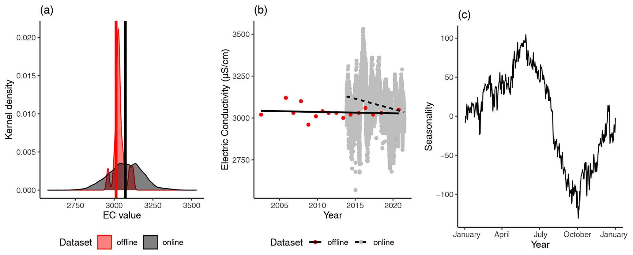
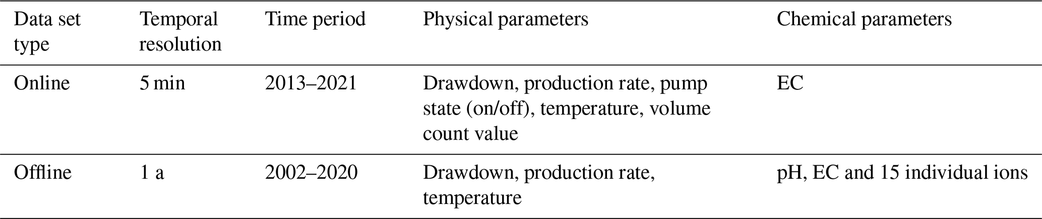
Figure 1(a) Density histograms of both online and offline data at BAK. (b) Timelines and linear trend lines of EC-concentrations calculated for online and offline data. The dashed line shows the trend for the online data set. The solid line indicates the trend line for the offline data set. (c) Seasonal component of time series decomposition analysis based on the online data set.
For the prediction of the development of the hydrochemical composition, an autoregressive integrated moving average (ARIMA) model forecast was chosen. This algorithm assumes the future value of a variable to be a linear function of a data time series' several past observations and random errors (Zhang, 2003). Due to its simplicity, it constitutes one of the most popular linear forecasting approaches (Ho and Xie, 1998; Zhang, 2003). We calculated the prognosis based on offline data by using the R function forecast::auto.arima (Hyndman et al., 2021), which automatizes the forecast given equidistant time series data. Equidistance in the data set was achieved, like before, through linear interpolation between neighboring analyses (stats::approx). Using the same method, a forecast based on the online data was produced to compare resulting value ranges.
In order to elevate information on individual hydrochemical constituents to seasonal development, we conducted multiple linear regression analyses to assess the potential of these data sets for use in virtual sensors. This was done with the aim of discerning relationships between offline and online data in order to extrapolate high temporal resolution values of parameters which can realistically only be measured on a low temporal resolution. In addition to the individual parameters we defined parameter groups and ratios: discerning dolomite vs. calcite inflow, and for discerning inflow of waters subject to ion exchange, to signal saline inflow dynamics, and Na+ + − for discerning saline versus ion exchange water inflow. The strongest correlations, as indicated by the Pearson correlation coefficient (PCC), were then further investigated through specific regression models. All regression models show a 0.99 confidence area and were computed using the default R package “stats” (R Core Team, 2020).
A calculation regarding mixing ratios was performed using the software PhreecC (Parkhurst and Appelo, 2013).
In this chapter, results for BAK will be shown in detail and important results from the analyses of BF2 (Figs. S1 and S2 in the Supplement) are briefly presented.
3.1 Time series analysis
The density graph in Fig. 1a) shows differences in value ranges between the offline and the online data sets. The vertical bars indicate the mean values for each data set, which lie at 3071.72 ± 109.63 µS cm−1 for online data, and at 3012.35 ± 97.63 µS cm−1 for offline data (1471.66 ± 135.02 and 1434.28 ± 38.05 µS cm−1 respectively for BF2). The overlapping kernel density curves show a more evenly distributed curve for the online data set compared to the offline data set. The larger SD for the online data set represents the larger variability shown in Fig. 1b) which depicts the two time series and trend lines calculated for each data set. Both data sets are characterized by a negative trend, however, while the offline data resulted in an almost even but minimally negative trend line, the trend derived from the online data set shows a clearly negative course. Although sampling period is considerably shorter for the online data, this does not explain the differences in trend. When we restricted the offline data to the same sampling period as the online data, the offline trend became very slightly positive. Thus, online and offline data systematically disagree on trend determination. In BF2, similar differences between the trend lines are observed, but in this case both trends are positive.
Time series decomposition resulted in Fig. 1c) which depicts the seasonal component for one year. A local maximum in late spring (104.36) and a local minimum in early autumn (−130.67) mark the seasonal variations. Obviously, offline data with yearly analyses can not exhibit any seasonal variations. BF2 did not show any clear seasonal variations.
Inter-annual fluctuations for eight individual ions (Na+, K+, Ca2+, Mg2+, F−, Cl−, and ) were also examined. Over a time span of 20 years, the hydrochemical analyses show little variation. The highest relative SD values are displayed by Ca2+ (23.18 %), K+ (20.50 %) and F− (20.39 %), all of which exhibit low concentrations compared to the main ingredients.
3.2 ARIMA forecasting
The ARIMA forecasts differ strongly for online and offline data. Fig. 2a) shows an ARIMA forecast produced on the basis of offline data. The online data is depicted on top of the offline data. This shows that the forecast projects an expected value range which includes the measured offline data, however, it fails to cover even the currently measured online data. On the other hand, Fig. 2b) shows the ARIMA forecast based on online data. The projected value range covers a significantly wider area than the forecast based on offline data. Neither forecasts are able to produce a clear trend.
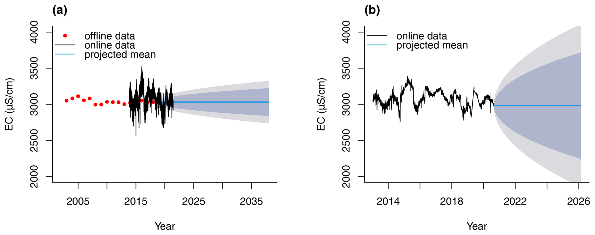
Figure 2ARIMA forecasts for EC values at BAK. The forecast ranges are depicted in light blue: 85 % confidence interval; light grey: 95 % confidence interval. (a) forecast based on offline EC data, as well as overlaid online EC data. (b) forecast based on online EC data.
3.3 Correlation analysis
Among the assessed ions and physical parameters, such as temperature, extraction volume and drawdown, we found several strong correlations as indicated by the PCC and visualized them in scatter plots (Fig. 3). Due to the small sample sizes, many of these correlations were not statistically significant (based on the p-value and a significance level of 0.05), however, it is still worth to explore them as they can offer valuable insights into important hydrogeochemical dynamics. We found the obvious strong connection between drawdown and extraction volume (R=0.93; Fig. 3a), but also between drawdown and EC (R=0.99; Fig. 3b). Variations in TDS are covered by the concentration values of bicarbonate (R=0.86) and sodium (R=0.90). None of the calculated ratios showed any strong correlations with the physical parameters (R>0.6) and only with their own constituents.
This study set out to compare the information values of offline and online data gathered for a geothermal well, assess whether the current practice of yearly hydrochemical sampling is an adequate strategy on which a robust assessment of the status-quo and reliable forecasts can be based, and to use strong correlations between the two data sets to assess the applicability of virtual sensors to this setting where offline data fell short of providing critical information. For this, we assumed that a well's hydrochemical signature indicates flow paths, and changes in its signature indicate changes in flow paths.
One of the most striking pieces of information produced by this study was the comparison of yearly data, which is the current sampling standard (e.g. in Germany as mandated by the German Spa Association (Länderarbeitsgemeinschaft für Wasser, 1998)), and online data measurements which still remain scarce. While one could argue that the data sets agree on similar mean EC values, they differ vastly in their covered time period, seasonality and trends (Fig. 1).
The higher variation in the online data is not caused by a change of the operation conditions of the well, which is evident from the data from 2013 to 2020. Information on operating conditions was provided by the operators of the well. Lockdowns due to Covid-19 only affected contained time spans in 2020 and there were extensions or changes made to the infrastructure of the medical spa. Accordingly, visitor numbers stayed relatively constant. It is interesting to note that the application type of the well is probably responsible for the amplitude of seasonal variations.
The seasonal fluctuations are controlled by changes in the spa operation: the number of visitors is highest in winter and spring and therefore the volume withdrawn is also higher for these seasons compared to summer months (Fig. 1c). In contrast, BF2 does not show seasonal variations in the same way, because the well produces water continuously for balneological uses and heating which leads to more constant production rates. On the other hand, it might also indicate less inflow from above and below (Fig. S1). However, most aquifers are structurally heterogeneous and connected to the adjacent strata above and below. Inflow from these strata is a function of pressure in the main aquifer, even if their connection is weak. Increasing production rates lead to a decrease in the pressure in the main aquifer, which results in a pressure gradient to the adjacent stratigraphic units. If the hydrochemical composition in these units is different from the main aquifer, or if the main aquifer is strongly heterogeneous, changes in TDS (measured by EC probes at the well head) are to be expected. However, this correlation shows temporal dependencies which span over long periods, i.e. correlation between production rate and EC differ depending on the production regime leading up to the sampling date. This is a clear sign that the offline data fail to represent the hydrochemical state of the groundwater well at seasonally varying operating conditions. An assessment based on offline data alone will thus underestimate the contribution of other strata to the main aquifer.
Variability of the online data does show changes within the recorded time span. This corresponds with the trends detected in both data sets which differ starkly (Fig. 1b).
Overall, by omitting sub-yearly, seasonal fluctuations, the offline data set merely offers a snapshot of the well's hydrochemical state. The snapshot is limited in its informative value to the sampling date and does not provide any information on between-sampling fluctuations. This can lead to misjudgments on the hydrochemical stability of the well and seasonal activation of additional inflow pathways. Time series decomposition derived a seasonal variation frequency of 1 year (Fig. 1b). Accordingly, the Nyquist-Theorem demands that the sampling frequency be higher than one sample every six months in order to adequately represent the fluctuations with a 12 month period. We thus suggest a sampling frequency of 4 to 5 months which is higher than the current practice of one sample a year, but lower than the suggested frequencies by Zhou (1996) of 1 month, and by Barcelona et al. (1989) of 2 to 3 months. Their high sampling frequencies are likely due to stronger sub-seasonal variations in shallow ground water aquifers, by which deep ground water aquifers, such as the one in this study, are less impacted. However, this study showed that clear seasonal variations can also be found in deep ground water aquifers. The proposed scheme is applicable to all deep groundwater wells except for cases where the confining layers prevent any inflow from above or below at the well and in its vicinity. In this case, the water originates only from the reservoir and will not show any change in the flow pattern due to changes.
Figure 3Selection of univariate regressions marked by a high Pearson correlation coefficients based on the offline data set at BAK. The blue line indicates the linear regression model, the grey shaded area shows the 99 % confidence interval.
We further demonstrated that the ARIMA forecast for EC values, built upon offline data, neglects to consider even currently observed, sub-yearly EC concentration fluctuations. Due to the sampling bias, the forecast based on offline data (Fig. 2a) shows a rather small prediction interval and no trend. This is in line with very little variations of the hydrochemical composition observed over the years. The forecast based on online data reveals a great uncertainty but still no trend. This indicates that changes in the flow patterns to this particular well are fully reversible and points to a hydraulic activation of flow paths in a heterogeneous reservoir, rather than an influx from overlying or underlying stratigraphic units as seen e.g. at the Pullach Th2 well (Baumann et al., 2017). Part of the uncertainty can also be attributed to the shorter time span of online data. In the case of this well, we showed conclusively that a forecast, as required for many deep ground water aquifers by the WFD, based on yearly measurements, fails to represent sub-yearly variations in EC, and only represents one very specific state of the well. Thus, forecasting needs to be conducted with higher-resolution data in order to take these developments into account.
Having shown that yearly groundwater sampling does not adequately represent real hydrochemical fluctuations in the reservoir, the possibilities of applying VS in this field were tested. While we found some correlations with a high PCC, the correlations were rarely statistically significant (Fig. 3). This is due to the small size of the available data sets. There was an expected correlation between the production rate (or drawdown) and temperature. The correlation between water temperature and TDS might point to different flow patterns. The correlation between EC and drawdown allowed insights into some hydrochemical dynamics. The hydrochemical signature of the two most divergent analyses in our correlation assessment show slightly lower TDS: Na+, Cl−, and show lower concentrations, K+, Ca2+, and show higher concentrations. Assuming a minor change of the flow pattern at high production rate with an influx of 7 % of another water type, the calculated inflow water is a K+ − Ca2+ − − − type with a TDS of 1100 mg L−1. The saturation indices calculated with PhreeqC show that the water is in equilibrium with dolomite, and under-saturated (saturation index = −1) with respect to gypsum. The calculated hydrochemistry of the in-flowing water does not fit waters of the crystalline basement or the overlying sandstones of the lower Jurassic (Carlé, 1975). Furthermore, the variations recorded by the online measurements are much larger compared to the analysis data. Therefore, the hydrochemistry of the in-flowing water would cause an even starker contrast to the assumed composition. Assuming a mix with 50 % of another water type leads to similar TDS and hydrochemical signature, and would indicate lithostratigraphic heterogeneity or hydrochemical stratification in the reservoir.
To make use of VS to span data gaps and assess dynamic changes of the inflow pathways to the well, a number of prerequisites have to be met. The relationships between offline and online data sets must be based on larger data sets than are currently available to ensure statistically significant correlations. However, stronger data might also include the following: ideally, flow-meter logs and/or fibre optical measurements (Schölderle et al., 2021) are available to define the immediate inflow zones to the well at different production rates. To assess inflow from adjacent strata, pumping tests during exploration or information from wells close by and reaching into these strata can provide relevant information. The relation between production rate and hydrochemical characteristics can be obtained from pumping tests with different production rates. Long-term hydrochemical data can provide information about inflow zones further away from the well. Finally, under ideal conditions, a hydrogeochemical model framework to assess the interactions and reactions of the (mixed) waters along the flow paths is available.
This study showed that on the basis of two wells, one which is solely used for balneological purposes, and one which is exploited for balneology and constant energy production, the current state of the art practice of yearly hydrochemical measurements fail to accurately represent trend, mean and seasonality. It is thus of great importance that more data with high temporal resolution is made available. Since direct physical measurements of the variables in question are financially and physically impossible, virtual sensors could offer a viable alternative. We thus conclude that:
-
Yearly samples taken at the same stress state are underestimating the hydrochemical variations of the produced waters. This is relevant for balneological and geothermal applications with regards to the legal framework pertaining to recognition as medical spas, and predictive maintenance and prevention of corrosion and scaling, respectively.
-
Basing hydrochemical forecasting algorithms, such as ARIMA, on yearly data did not result in reliable value ranges. The calculated ranges failed to include even currently measured sub-yearly signal response variability when used on EC data.
-
Online data provide quantitative access to the nature of the processes responsible for changes in the hydrochemical conditions, and whether they are reversible or not. However, online data require careful hydrochemical characterization of the well (hydrochemical pumping tests, hydrochemical and hydraulic logs, depth oriented sampling) to make full use of their predictive potential, e.g. use in VS applications.
Knowing the precise fluctuations of the individual ions, TDS and overall hydrochemical composition is important knowledge for predictive maintenance and serves as an indicator and warning signal for unsustainable groundwater extraction schemes. For this, we estimate that sensor fusion in the framework of geothermal science is possible if there is a proper prior characterization of the reservoir, and the hydrochemical characteristics in the different parts of the reservoir are known. In order to achieve larger training data sets, it is crucial that hydrochemical assessments take place more often than once a year.
Overall, more frequent sampling at different production scenarios, and learning algorithms in combination with mixing models will aid implementing VS to the field of geothermal water production.
All code was written using the statistical software R and is available on request. The software as well as the relevant clustering packages can be downloaded under https://www.r-project.org/ (last access: 16 December 2022). Hydrochemical data is available on request.
The supplement related to this article is available online at: https://doi.org/10.5194/adgeo-58-189-2023-supplement.
TB conceived the presented idea. AD developed the theory and performed the computations. TB verified the analytical methods and supervised the findings of this work. Both authors discussed the results and contributed to the final manuscript. AD wrote the manuscript with support from TB.
The contact author has declared that none of the authors has any competing interests.
This article is part of the special issue “European Geosciences Union General Assembly 2022, EGU Division Energy, Resources & Environment (ERE)”. It is a result of the EGU General Assembly 2022, Vienna, Austria, 23–27 May 2022.
Publisher’s note: Copernicus Publications remains neutral with regard to jurisdictional claims in published maps and institutional affiliations.
The authors would like to thank the reviewers and Ingrid Stober (Karlsruhe Institute of Technology) for their very helpful comments and the operators of the wells BAK and BF2 for supplying data. We also would like to thank the lab technicians Birgit Apel and Joachim Langer.
This study was funded by the Bavarian State Ministry of Science, Research and Art in the Framework of the Geothermal-Alliance Bavaria.
This work was supported by the Technical University of Munich (TUM) in the framework of the Open Access Publishing Program.
This paper was edited by Gregor Giebel and reviewed by two anonymous referees.
Alley, W. M., Bair, E. S., and Wireman, M.: “Deep” Groundwater, Groundwater, 51, 653–654, https://doi.org/10.1111/gwat.12098, 2013. a
Barcelona, M., Wehrmann, H., Schock, M., Sievers, M., and Karny, J.: Sampling Frequency for groundwater Quality Monitoring, US Environmental Protection, Office of Research and Development, Environmental Monitoring Systems Laboratory, EPA/600/4-89/032, 1989. a, b, c, d, e
Baumann, T., Bartels, J., Lafogler, M., and Wenderoth, F.: Assessment of heat mining and hydrogeochemical reactions with data from a former geothermal injection well in the Malm Aquifer, Bavarian Molasse Basin, Germany, Geothermics, 66, 50–60, https://doi.org/10.1016/j.geothermics.2016.11.008, 2017. a, b
Birner, J.: Hydrogeologisches Modell des Malmaquifers im Süddeutschen Molassebecken, PhD thesis, https://refubium.fu-berlin.de/handle/fub188/1492 (last access: 12 May 2023), 2013. a
Birner, J., Mayr, C., Thomas, L., Schneider, M., Baumann, T., and Winkler, A.: Hydrochemie und Genese der tiefen Grundwässer des Malmaquifers im bayerischen Teil des süddeutschen Molassebeckens Hydrochemistry and evolution of deep groundwaters in the Malm aquifer in the bavarian part of the South German Molasse Basin, Z. Geol. Wiss., 39, http://www.zgw-online.de/en/media/291-113.pdf (last access: 12 May 2023), 2011. a, b
Caers, J. and Castro, S.: A Geostatistical Approach to Integrating Data From Multiple and Diverse Sources: An Application to the Integration of Well Data, Geological Information, 3d/4d Geophysical and Reservoir-Dynamics Data in a North-Sea Reservoir, Subsurf. Hydrol. Data Integr. Prop. Process. Geophys. Monogr. Ser., 171, https://doi.org/10.1029/171GM07, 2006. a
Carlé, W.: Die Mineral- und Thermalwässer von Mitteleuropa: Geologie, Chemismus, Genese, Wissenschaftliche Verlagsgesellschaft, Stuttgart, ISBN 3 80470461 1, 1975. a, b
Deutscher Heilbäderverband and Deutscher Tourismusverband: Begriffsbestimmungen/Qualitätsstandards für Heilbäder und Kurorte, Luftkurorte, Erholungsorte – einschließlich der Prädikatisierungsvoraussetzungen – sowie für Heilbrunnen und Heilquellen, Tech. Rep., Deutscher Tourismusverband e.V. und Deutscher Heilbäderverband e.V., 2016. a
European Parliament and Council: Directive 2000/60/EC I – The European Water Framework Directive, https://doi.org/10.2779/75229, 2000. a, b
Hebig, K. H., Ito, N., Scheytt, T., and Marui, A.: Review: Deep groundwater research with focus on Germany, Hydrogeol. J., 20, 227–243, https://doi.org/10.1007/s10040-011-0815-1, 2012. a, b
Heine, F., Zosseder, K., and Einsiedl, F.: Hydrochemical Zoning and Chemical Evolution of the Deep Upper Jurassic Thermal Groundwater Reservoir Using Water Chemical and Environmental Isotope Data, Water, 13, 1162, https://doi.org/10.3390/w13091162, 2021. a
Ho, S. L. and Xie, M.: The use of ARIMA models for reliability forecasting and analysis, Comput. Ind. Eng., 35, 213–216, https://doi.org/10.1016/s0360-8352(98)00066-7, 1998. a
Hyndman, R., Athanasopoulos, G., Bergmeir, C., Caceres, G., Chhay, L., O'Hara-Wild, M., Petropoulos, F., Razbash, S., Wang, E., and Yasmeen, F.: forecast: Forecasting functions for time series and linear models, R package version 8.15, https://pkg.robjhyndman.com/forecast/ (last access: 16 December 2022), 2021. a
Kabadayi, S., Pridgen, A., and Julien, C.: Virtual sensors: Abstracting data from physical sensors, Proc. – WoWMoM 2006 2006 Int. Symp. a World Wireless, Mob. Multimed. Networks, 2006, 587–592, https://doi.org/10.1109/WOWMOM.2006.115, 2006. a
Kang, M., Ayars, J. E., and Jackson, R. B.: Deep groundwater quality in the southwestern United States, Environ. Res. Lett., 14, 034004, https://doi.org/10.1088/1748-9326/aae93c, 2019. a
Käss, W. and Käss, H.: Deutsches Bäderbuch, Schweizerb. Edn., ISBN 978-3-510-65241-9, 2008. a, b, c
Krieger, M., Kurek, K. A., and Brommer, M.: Global geothermal industry data collection: A systematic review, Geothermics, 104, 102457, https://doi.org/10.1016/j.geothermics.2022.102457, 2022. a, b
Länderarbeitsgemeinschaft für Wasser: Richtlinien für Heilquellenschutzgebiete, ISBN 3-88961-217-2, 1998. a
Martin, D., Kühl, N., and Satzger, G.: Virtual Sensors, Bus. Inf. Syst. Eng., 63, 315–323, https://doi.org/10.1007/s12599-021-00689-w, 2021. a
Mayrhofer, C., Niessner, R., and Baumann, T.: Hydrochemistry and hydrogen sulfide generating processes in the Malm aquifer, Bavarian Molasse Basin, Germany, Hydrogeol. J., 22, 151–162, https://doi.org/10.1007/s10040-013-1064-2, 2014. a
Nelson, J. D. and Ward, R. C.: Statistical Considerations and Sampling Techniques for Ground-Water Quality Monitoring, Ground Water, 19, 617–625, https://doi.org/10.1111/j.1745-6584.1981.tb03516.x, 1981. a
Parkhurst, D. L. and Appelo, C. A. J.: Description of input and examples for PHREEQC versoin 3: a computer program for speciation, batch-reaction, one-dimensional transport, and inverse geochemical calculations, in: Model. Tech., Chap. 43, U.S. Geological Survey, Reston, Virginia, https://doi.org/10.3133/tm6A43, 2013. a
Porter, D. W., Gibbs, B. P., Jones, W. F., Huyakorn, P. S., Hamm, L. L., and Flach, G. P.: Data fusion modeling for groundwater systems, J. Contam. Hydrol., 42, 303–335, https://doi.org/10.1016/S0169-7722(99)00081-9, 2000. a, b, c
R Core Team: R: a language and environment for statistical computing, https://www.r-project.org/ (last access: 16 December 2022), 2020. a, b
Schölderle, F., Lipus, M., Pfrang, D., Reinsch, T., Haberer, S., Einsiedl, F., and Zosseder, K.: Monitoring cold water injections for reservoir characterization using a permanent fiber optic installation in a geothermal production well in the Southern German Molasse Basin, Vol. 9, Springer Berlin Heidelberg, https://doi.org/10.1186/s40517-021-00204-0, 2021. a
Tegen, A., Davidsson, P., Mihailescu, R. C., and Persson, J. A.: Collaborative sensing with interactive learning using dynamic intelligent virtual sensors, Sensors (Switzerland), 19, https://doi.org/10.3390/s19030477, 2019. a
Zhang, P. G.: Time series forecasting using a hybrid ARIMA and neural network model, Neurocomputing, 50, 159–175, https://doi.org/10.1016/S0925-2312(01)00702-0, 2003. a, b
Zhou, Y.: Sampling frequency for monitoring the actual state of groundwater systems, J. Hydrol., 180, 301–318, https://doi.org/10.1016/0022-1694(95)02892-7, 1996. a, b, c, d