 | 03 Nov 2021
Evaluation of subseasonal to seasonal forecasts over India for renewable energy applications
Aheli Das
This study evaluates subseasonal to seasonal scale (S2S) forecasts of meteorological variables relevant for the renewable energy (RE) sector of India from six ocean-atmosphere coupled models: ECMWF SEAS5, DWD GCFS 2.0, Météo-France's System 6, NCEP CFSv2, UKMO GloSea5 GC2-LI, and CMCC SPS3. The variables include 10 m wind speed, incoming solar radiation, 2 m temperature, and 2 m relative humidity because they are critical for estimating the supply and demand of renewable energy. The study is conducted over seven homogenous regions of India for 1994–2016. The target months are April and May when the electricity demand is the highest and June–September when the renewable resources outstrip the demand. The evaluation is done by comparing the forecasts at 1, 2, 3, 4, and 5-months lead-times with the ERA5 reanalysis spatially averaged over each region. The fair continuous ranked probability skill score (FCRPSS) is used to quantitatively assess the forecast skill. Results show that incoming surface solar radiation predictions are the best, while 2 m relative humidity is the worst. Overall SEAS5 is the best performing model for all variables, for all target months in all regions at all lead times while GCFS 2.0 performs the worst. Predictability is higher over the southern regions of the country compared to the north and north-eastern parts. Overall, the quality of the raw S2S forecasts from numerical models over India are not good. These forecasts require calibration for further skill improvement before being deployed for applications in the RE sector.
- Article
(1592 KB) - Full-text XML
- BibTeX
- EndNote


The subseasonal to seasonal scale, also known as the S2S scale, with lead times extending from two weeks to a season (Vitart et al., 2017), is a new frontier in operational weather and climate prediction. S2S predictions can be beneficial in providing early warnings of extreme weather events and can aid in managing energy, agricultural, and hydrological resources (White et al., 2017). With most countries moving away from fossil fuels, renewable energy (RE) now accounts for 29 % of the global electricity generation (IEA, 2021). Unlike fossil fuels, RE resources are intermittent due to weather variability (Pechlivanidis et al., 2019). Forecasts can help the RE industry manage the intermittency. For example, wind speed and incoming solar radiation forecasts can help estimate future RE generation while temperature and humidity forecasts can help estimate future electricity demand. Forecasts of these variables at S2S scale are particularly important for RE producers, grid operators and energy traders for operations and maintenance scheduling, strategic planning and making investment decisions (Orlov et al., 2020).
Recognizing the value of S2S forecasts, many agencies provide operational S2S forecasts in the public domain. However, only a few studies focus on the assessment of S2S forecasts of RE variables obtained from numerical models. Lynch et al. (2014) analyzed weekly mean wind speeds over Europe from ECMWF 32 d forecast model and found evidence of skill beyond the medium range time scale. Marcos et al. (2018) characterized the global distribution of 10 m wind speeds forecasts from ECMWF System 4 with respect to ERA-Interim reanalysis in terms of mean, standard deviation, skewness, kurtosis, goodness-of-fit. They concluded that although the forecast could approximately represent the pattern of the mean and standard deviation of the reanalysis, it could not correctly replicate the patterns of the other moments. De Felice et al. (2019) transformed incoming solar radiation forecasts from ECMWF System 4 to forecasts of solar photovoltaic (PV) power potential over Europe. They found that the transformed forecasts showed some skill in predicting above and below normal PV power potential in certain European regions. Bell and Kirtman (2019) developed a grand multimodel ensemble (GMME) for forecasting 10 m wind speeds over the North Atlantic Ocean during the winter season. They found that eliminating some models helped to improve the GMME forecast skill. Prodhomme et al. (2021) investigated the ability of ECMWF SEAS5 model to predict seasonal summer heatwaves over Europe and discovered that the model performed better at grid-point level rather than at a regional level. In order to further improve the forecast quality by adjusting systematic errors (Doblas-Reyes et al., 2013), these raw forecasts undergo calibration. Calibrated forecasts of RE variables thus help to provide a better estimate of energy demand, wind, and solar energy production (Lledó et al., 2019; Soret et al., 2019; Bloomfield et al., 2021). These limited studies show that S2S forecasts have the potential to be exploited for RE applications.
Presently India is experiencing a remarkable growth in the RE sector. As of February 2021, India's RE capacity is 92.97 GW (MNRE, 2021). The Government of India plans to reach 227 GW of RE capacity by 2022 (PIB, 2019). High-quality S2S forecasts for the RE sector can play a significant role in aiding this growth. In spite of their availability, S2S forecast performance for RE variables has not been rigorously evaluated over India. Therefore, the objective of this study is to assess the performance of S2S forecasts of 10 m wind speed (WS10 m), incoming shortwave radiation at surface (SSW), 2 m temperature (T2 m), and 2 m relative humidity (RH2 m) from 6 ocean-atmosphere coupled models over India.
2.1 Forecast models
Monthly mean forecasts from six ocean-atmosphere coupled models are used in this study. The models are ECMWF SEAS5 (Johnson et al., 2019), DWD GCFS 2.0 (Fröhlich et al., 2021), Météo-France's System 6 (MF-6; Meteo-France, 2017), NCEP CFSv2 (Saha et al., 2014), UKMO GloSea5-GC2-LI (GS5-GC2-LI; MacLachlan et al., 2014), and CMCC SPS3 (Sanna et al., 2017). The forecasts are available on the C3S Climate Data Store (CDS, 2021). For brevity, only a brief summary of the models are provided in Table 1. Detailed information is available in the references cited above.
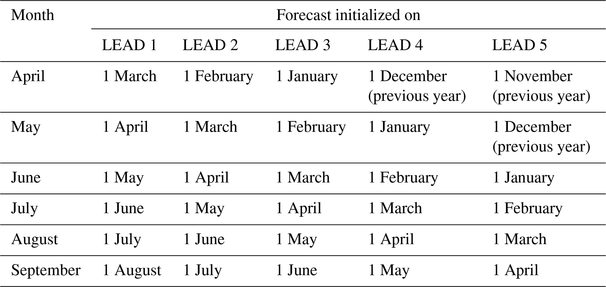
The models are run over a global domain with a 1∘ × 1∘ resolution. The ensemble members of SEAS5, GCFS 2.0, SPS3 are initialized in a burst mode, whereas MF-6, CFSv2, and GloSea5-GC2-LI are initialized in a lagged mode. In burst mode, all ensemble members are initialized at the same time with slightly varying initial conditions, whereas, in a lagged mode, the ensemble members are initialized at different times (Vitart and Takaya, 2021). But the monthly datasets in Climate Data Store are encoded such that all the members in lagged mode are initialized on the 1st of every month. Based on this, the initialization time of every target month in this study is mentioned in Table 2.

2.2 Study area and period
The forecast models are evaluated over the seven homogenous regions of India (Fig. 1). They are western Himalayas (WH), north west (NW), north central (NC), north east (NE), interior peninsula (IP), west coast (WC), and east coast (EC). The regions are demarcated based on climate, geography, and topography (Kothawale and Rupa Kumar, 2005). The study period spans from 1994 to 2016, which is the common hindcast period of all the models. The study is conducted over two interesting time periods: (i) summer months of April, May when the electricity demand is high (POSOCO, 2016), and (ii) monsoon months of June, July, August, and September when the supply of renewable resources is higher than the demand (Dunning et al., 2015).

Figure 1Homogenous regions of India.
2.3 Observations
ERA5 reanalysis (Hersbach et al., 2020) is used as the observational reference. This latest reanalysis dataset produced by ECMWF has replaced ERA-Interim and spans from 1950 to the present. Similar to the forecasts, the reanalysis is also retrieved from C3S Climate Data Store. ERA5 is produced using 4D-Var data assimilation in IFS Cycle41r2. The high resolution hourly dataset has a 31 km horizontal resolution and 137 vertical levels up to 0.01 hPa. We perform bilinear interpolation on the reanalysis to bring it to the same 1∘ × 1∘ resolution as the forecasts. The 2 m relative humidity is calculated from 2 m temperature and 2 m dew point temperature using an improved Magnus formula (Alduchov and Ecksridge, 1996). Both the forecasts and reanalysis are extracted over each homogenous region and then spatially averaged. We use these extracted values to calculate the verification metric.
2.4 Verification metric
Continuous ranked probability skill score (CRPSS; Wilks, 2019) is used as the measure of forecast skill. It is a probabilistic skill score that measures the difference between observed and predicted cumulative distributions with respect to climatology. But the CRPSS can give unfair results when comparing forecasts from different models with a different number of ensemble members. Therefore, the fair version of CRPSS (Ferro et al., 2008), known as FCRPSS, is used as the unbiased measure of probabilistic forecast skill. The climatology of the variables for each region is obtained from ERA5. The FCRPSS is calculated for each variable, model, target month, region, and lead time using the SpecsVerification package in R (Siegert, 2020). FCRPSS = 1 indicates that the forecasts are perfect, FCRPSS = 0 suggests that the forecast skill is the same as climatology, and FCRPSS < 0 means that the forecasts are worse than climatology. A forecast is considered skilful if the FCRPSS is greater than 0.
Our forecast dataset has 4 variables, 6 models, 6 target months, 7 regions, and 5 lead times giving a total of 5040 combinations. The forecasts are evaluated for each of these 5 parameters. Out of the 5040 forecasts, only 1302, that is 25.8 % of the total, are skilful. Figure 2 shows the distribution of FCRPSS values. The FCRPSS values in the x-axis are separated into bins of width 0.1, and the y-axis displays the number of forecasts for each bin. Most of the skilful values are in the range 0.1 to 0.4, with only a few greater than 0.4. This suggests that even though some of the predictions possess a certain degree of skill, they are far from perfect.
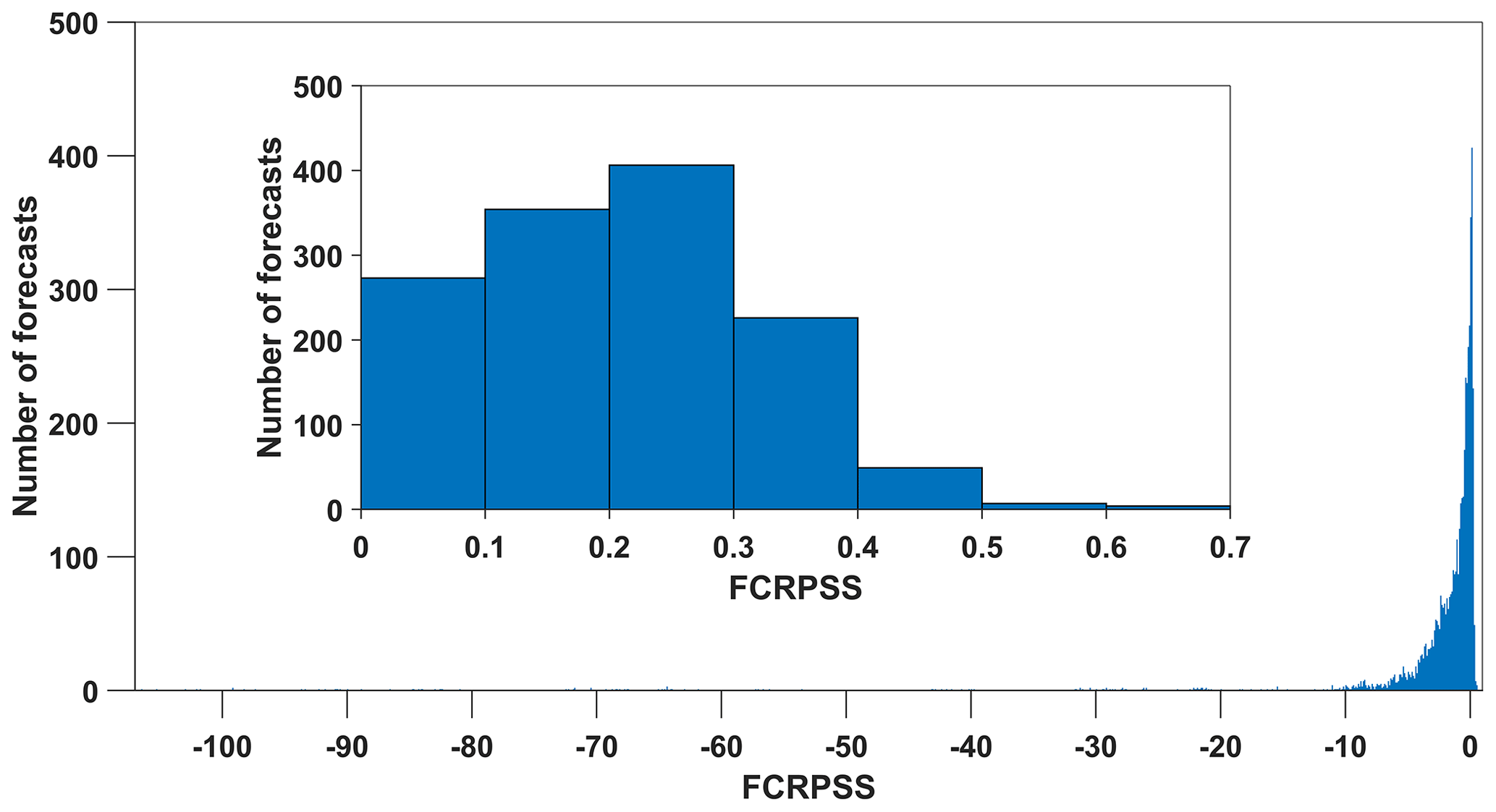
Figure 2Bar plot showing the distribution of all 5040 FCRPSS values. FCRPSS values are in the range [−106.38, 0.63]. Inset bar plot shows the distribution of only the 1302 forecasts that are skilful with FCRPSS > 0.
Given the 5 different parameters that are used in this study, a combination of smaller subset of these parameters will result in different number of forecasts. Table 3 shows the number of forecasts that result when a combination of any 2 parameters out of total 5 are chosen for analysis.
Table 3Number of forecasts for different combinations of the parameters used in this study.

Figure 3 depicts the performance of forecasts for the four variables in different models, regions, target months, and lead times. Figure 3a shows that SEAS5 is the best performing model while GCFS2.0 is the worst. Performance for all variables is the best in SEAS5. Forecast skill for T2 m and WS10 m are the worst in GCFS 2.0 whereas, SSW and RH2 m skill are worst in GS5-GC2-LI. SSW is the best predicted variable and RH2 m is the worst. Figure 3b shows that forecast skill for T2 m is better in the summer but worse in the monsoon. The reverse is true for WS10 m, SSW, and RH2 m. Figure 3c shows that predictability over three southern regions (IP, WC, EC) is very high, but it is pretty low over WH except for SSW. Finally, Fig. 3d indicates that RH2 m show a sharp decline in forecast skill with increasing lead time but the skills for other variables remain more or less the same.
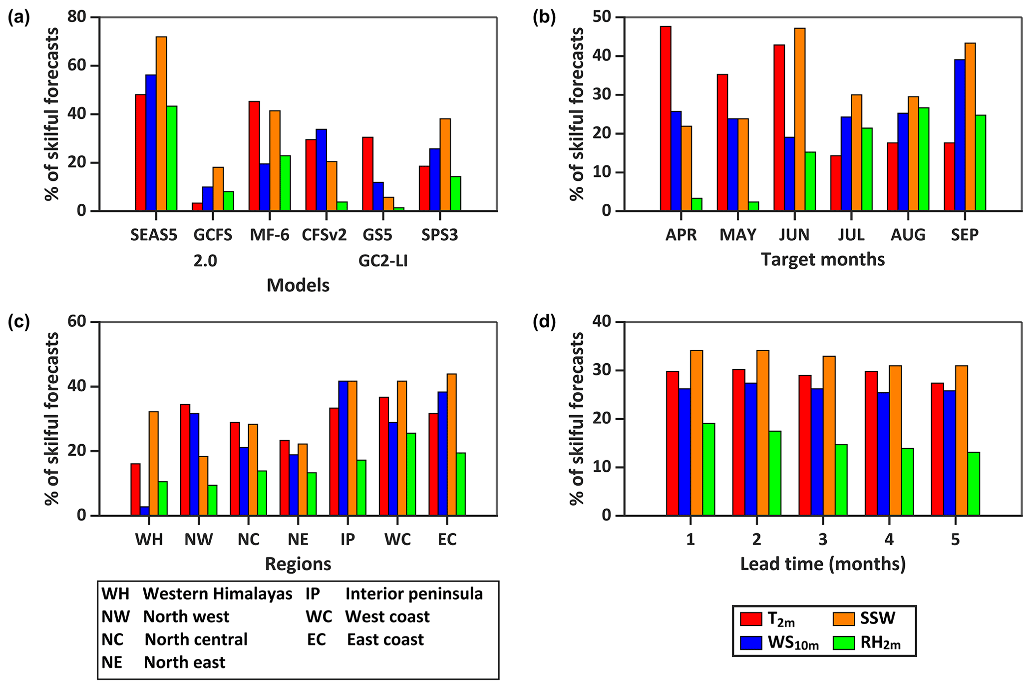
Figure 3(a) Forecast performance for variables in different models. (b) Forecast performance for variables in different target months. (c) Forecast performance for variables in different regions. (d) Forecast performance for variables at different lead times.
Figure 4 displays the forecast performance for the models in different target months, regions, and lead times. Figure 4a shows that SEAS5 performs the best at all the target months, while GCFS 2.0 and GS5-GC2-LI perform the worst. From Fig. 4b, SEAS5 shows the highest skill over all the regions. Furthermore, most models show greater skill over IP, WC, and EC than over WH, NW, NC, and NE. Figure 4c reveals that SEAS5 performance stands apart from the rest at all lead times. Forecast performance remains more or less similar across lead times except for CFSv2 that shows reduced skill with increased lead time. Interestingly, MF-6 shows the lowest skill at 1-month lead time.
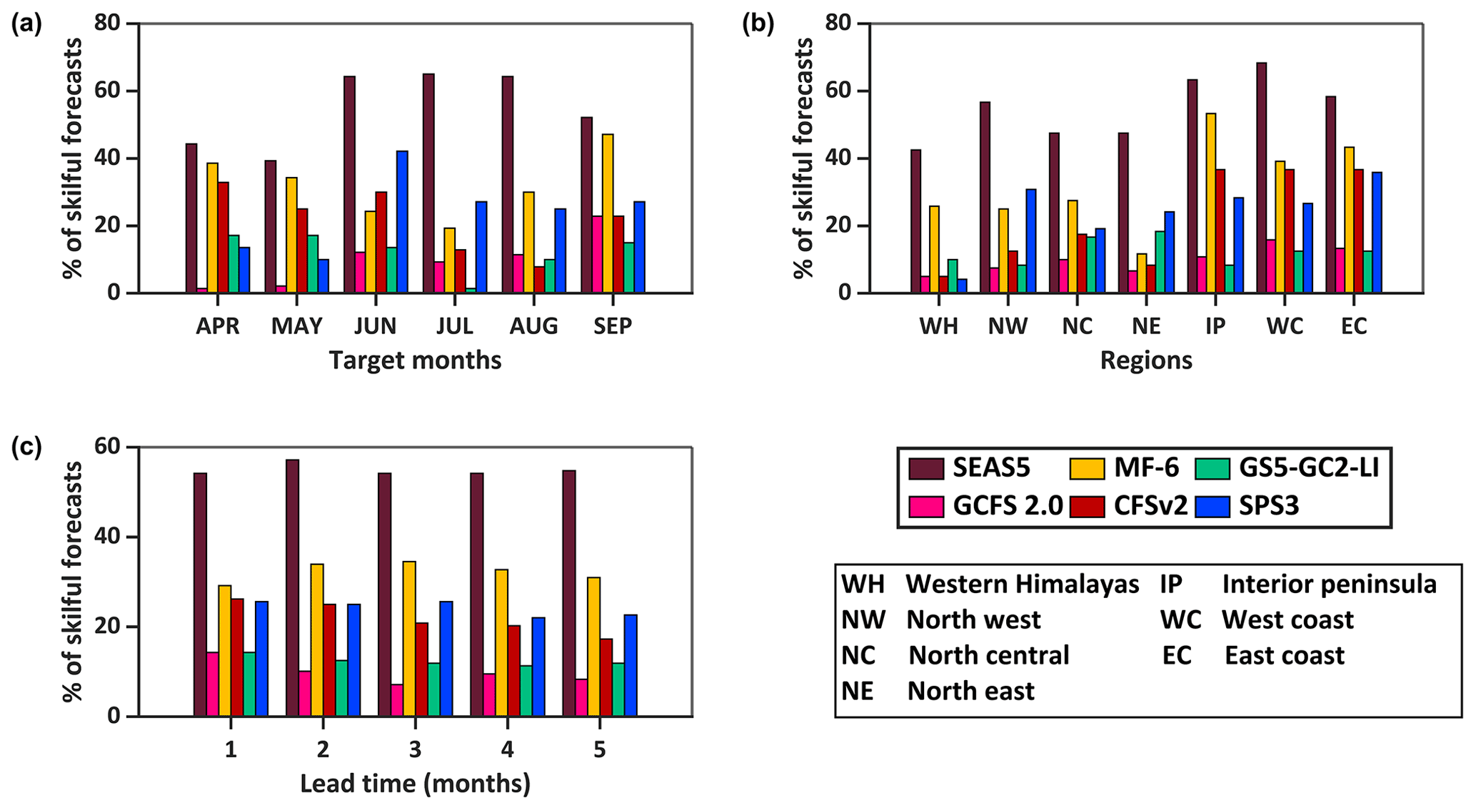
Figure 4(a) Forecast performance for models in different target months. (b) Forecast performance for models in different regions. (c) Forecast performance for models at different lead times.
Figure 5 shows the forecast performance for target months in different regions and lead times. Figure 5a shows that the predictability over the southern regions (IP, WC, EC) is high at all the target months as also evident in Fig. 4b. WH and NE have a poor predictability, except during June when the forecast skills are comparable with other regions. From Fig. 5b, it can be seen that forecast skills for April–June show a declining trend with increasing lead time whereas skills for July–September show a peak at 2–3 month lead times.
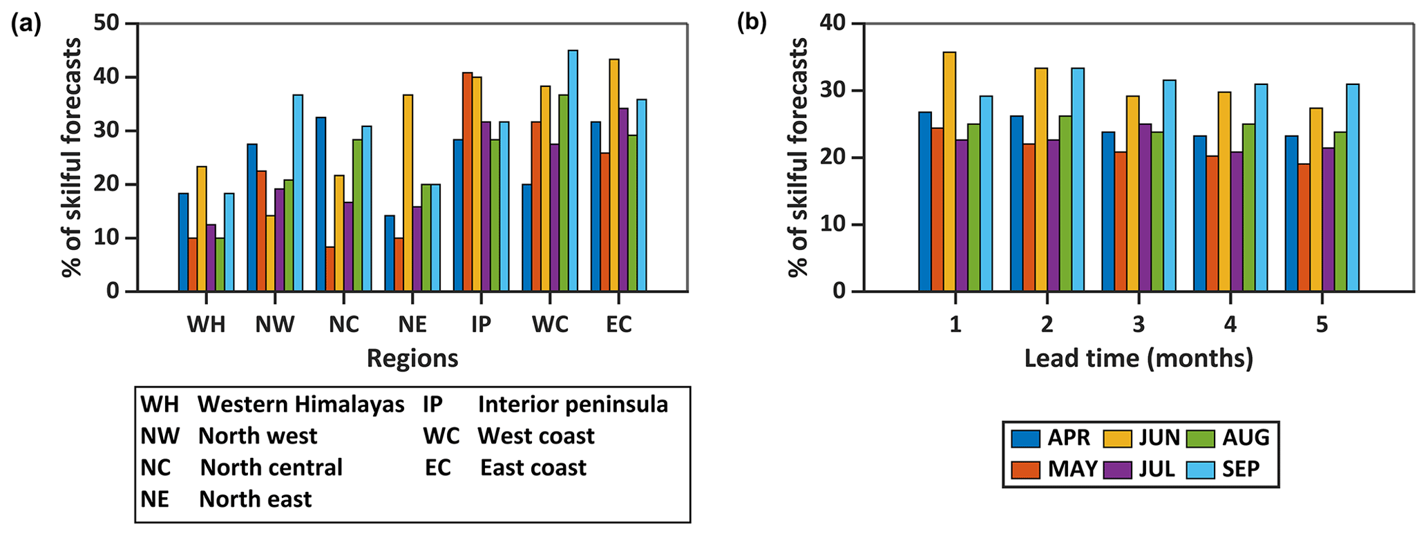
Figure 5(a) Forecast performance for target months in different regions. (b) Forecast performance for target months at different lead times.
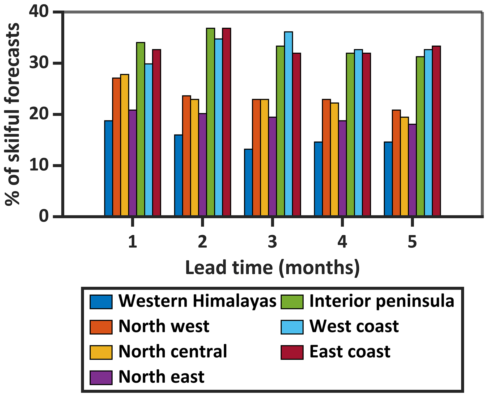
Figure 6 demonstrates the forecast performance for homogenous regions at different lead times. It shows that the predictability over the northern regions (WH, NW, NC, NE) is highest at lead time 1, whereas over the southern regions (IP, WC, EC), the predictability at lead time 2 is higher.
This study evaluates forecast skills of 4 meteorological variables relevant for the RE sector from 6 ocean-atmosphere coupled models over 7 homogenous regions of India using FCRPSS. The key conclusions of this study are:
-
Overall forecast performance in the S2S scale over India is poor. FCRPSS values for all parameters combined rarely exceed 0.4.
-
Forecast performance for SSW is the best, while that for RH2 m is the worst.
-
SEAS5 is the best performing model for all variables for all target months in all regions for all lead times. GCFS 2.0 performs the worst.
-
September has the highest number of skilful forecasts while May has the least.
-
The predictability is higher over the southern regions of the country compared to the north and north-eastern parts.
-
Predictability does not appreciably change with lead time except for RH2 m where predictability degrades with increasing lead time.
Because of the large number of parameters involved, it is challenging to find causal relationships to explain each and every signal. Nonetheless, we can speculate on some interesting patterns. For example, forecast performance for SSW, WS10 m and RH2 m is better in the monsoon season. This indicates that the models are able to simulate the synoptic scale features associated with the monsoons better than the finer scale convective phenomena that govern the pre-monsoon meteorology over India. Perhaps improving the resolution of the models or their subgird parameterization may lead to improvement in the pre-monsoon forecasts.
Regional drivers play an important role in forecast performance. Vicinity to the oceans favors the forecast skill for the southern regions of the country (IP, WC, EC). Apart from regulating the temperature over these regions due to its high heat capacity, the oceans also provide and retains predictable signals through SST anomalies for extended time periods. Perhaps the better representation of these processes by the models also explains why a higher skill is observed at lead times 2 or 3 instead of lead time 1 over these regions. The primary reason behind the poor forecast skill for most variables over western Himalayas is the inadequate representation of sub-grid scale orography, such as the distribution and alignment of mountain slopes and valleys that leads to poor wind speeds forecasts. On the other hand, radiation forecasts in this region are skilful, possibly due to the lack of aerosols at such heights.
Our results show that forecast performance does not appreciably degrade with time, which appears to be counterintuitive. The ensemble members of these S2S predictions deal with all possible states of evolution of the coupled model and thereby retain some skill that does not decline rapidly with lead time unlike a single deterministic prediction. A study by Chen et al. (2010) reported a similar finding that monthly mean temperature forecasts at lead times of 1 month and beyond reach a near constant value in the tropics where SST anomalies induce predictability. Therefore, the horizon of skilful forecasts, especially in the tropics, is largely determined by the ability of the S2S models to properly simulate large scale ocean-atmosphere circulation features like ENSO, MJO, and IOD and their teleconnections due to their influence on global weather patterns.
Further work is required to establish causal relationships behind our findings. Of particular importance is to identify the ability of the models and the parameterizations involved to simulate earth system phenomena like ENSO, IOD, and MJO that aid in long-term predictability. Nonetheless, this study shows that raw S2S forecasts from numerical models have some skill. This limited skill is a result of systemic errors in the model such as poor formulation of physical processes, poor initial conditions, limited resolution of the models and so on (Doblas-Reyes et al., 2013). Calibrating these forecasts with respect to a reference observation will make them closely resemble the observations by adjusting different moments of the forecast distribution, thereby minimizing the errors and enhancing the forecast skill. The fact that these evaluated forecasts already possess a certain amount of skill gives hope that calibration will add more value and upgrade their quality. The calibrated S2S forecasts will then be suitable for utilization by stakeholders in the RE industry for real-world applications.
Monthly forecasts were downloaded from the Copernicus Climate Change Service (C3S) Climate Data Store (CDS) (https://cds.climate.copernicus.eu/cdsapp#!/dataset/seasonal-monthly-single-levels?tab=form, CDS, 2021). ERA5 monthly averaged data were also downloaded from the Copernicus Climate Change Service (C3S) Climate Data Store (CDS) (https://doi.org/10.24381/cds.f17050d7, Hersbach et al., 2019).
AD and SBR conceptualized the study. AD conducted the analysis. AD and SBR wrote the paper.
The contact author has declared that neither they nor their co-author has any competing interests.
Publisher's note: Copernicus Publications remains neutral with regard to jurisdictional claims in published maps and institutional affiliations.
This article is part of the special issue “European Geosciences Union General Assembly 2021, EGU Division Energy, Resources & Environment (ERE)”. It is a result of the EGU General Assembly 2021, 19–30 April 2021.
This paper is partially funded by the ReNew Power Centre of Excellence for Energy and Environment vide Grant RP03241/MI02349. Aheli Das was financially supported by a Junior Research Fellowship (File no. 09/086(1401)/2019-EMR-I) from the Council of Scientific and Industrial Research (CSIR), New Delhi.
This paper was edited by Gregor Giebel and reviewed by two anonymous referees.
Alduchov, O. and Eskridge, R.: Improved Magnus Form Approximation of Saturation Vapor Pressure, J. Appl. Meteorol., 35, 601–609, https://doi.org/10.1175/1520-0450(1996)035<0601:imfaos>2.0.co;2, 1996.
Bell, R. and Kirtman, B.: Seasonal Forecasting of Wind and Waves in the North Atlantic Using a Grand Multimodel Ensemble, Weather Forecast., 34, 31–59, https://doi.org/10.1175/waf-d-18-0099.1, 2019.
Bloomfield, H. C., Brayshaw, D. J., Gonzalez, P. L. M., and Charlton-Perez, A.: Sub-seasonal forecasts of demand and wind power and solar power generation for 28 European countries, Earth Syst. Sci. Data, 13, 2259–2274, https://doi.org/10.5194/essd-13-2259-2021, 2021.
CDS: Seasonal forecast monthly statistics on single levels, Copernicus Climate Change Service (C3S) Climate Data Store (CDS) [data set], available at: https://cds.climate.copernicus.eu/cdsapp#!/dataset/seasonal-monthly-single-levels?tab=form, last access: 6 March 2021.
Chen, M., Wang, W., and Kumar, A.: Prediction of Monthly-Mean Temperature: The Roles of Atmospheric and Land Initial Conditions and Sea Surface Temperature, J. Climate, 23, 717–725, https://doi.org/10.1175/2009jcli3090.1, 2010.
De Felice, M., Soares, M., Alessandri, A., and Troccoli, A.: Scoping the potential usefulness of seasonal climate forecasts for solar power management, Renew. Energ., 142, 215–223, https://doi.org/10.1016/j.renene.2019.03.134, 2019.
Doblas-Reyes, F., García-Serrano, J., Lienert, F., Biescas, A., and Rodrigues, L.: Seasonal climate predictability and forecasting: status and prospects, WIREs Clim. Change, 4, 245–268, https://doi.org/10.1002/wcc.217, 2013.
Dunning, C., Turner, A., and Brayshaw, D.: The impact of monsoon intraseasonal variability on renewable power generation in India, Environ. Res. Lett., 10, 064002, https://doi.org/10.1088/1748-9326/10/6/064002, 2015.
Ferro, C., Richardson, D., and Weigel, A.: On the effect of ensemble size on the discrete and continuous ranked probability scores, Meteorol. Appl., 15, 19–24, https://doi.org/10.1002/met.45, 2008.
Fröhlich, K., Dobrynin, M., Isensee, K., Gessner, C., Paxian, A., Pohlmann, H., Haak, H., Brune, S., Früh, B., and Baehr, J.: The German Climate Forecast System: GCFS, J. Adv. Model. Earth Sy., 13, e2020MS002101, https://doi.org/10.1029/2020ms002101, 2021.
Hersbach, H., Bell, B., Berrisford, P., Biavati, G., Horányi, A., Muñoz Sabater, J., Nicolas, J., Peubey, C., Radu, R., Rozum, I., Schepers, D., Simmons, A., Soci, C., Dee, D., and Thépaut, J.-N.: ERA5 monthly averaged data on single levels from 1979 to present, Copernicus Climate Change Service (C3S) Climate Data Store (CDS) [data set], https://doi.org/10.24381/cds.f17050d7, 2019.
Hersbach, H., Bell, B., Berrisford, P., Hirahara, S., Horányi, A., Muñoz-Sabater, J., Nicolas, J., Peubey, C., Radu, R., Schepers, D., Simmons, A., Soci, C., Abdalla, S., Abellan, X., Balsamo, G., Bechtold, P., Biavati, G., Bidlot, J., Bonavita, M., Chiara, G., Dahlgren, P., Dee, D., Diamantakis, M., Dragani, R., Flemming, J., Forbes, R., Fuentes, M., Geer, A., Haimberger, L., Healy, S., Hogan, R., Hólm, E., Janisková, M., Keeley, S., Laloyaux, P., Lopez, P., Lupu, C., Radnoti, G., Rosnay, P., Rozum, I., Vamborg, F., Villaume, S., and Thépaut, J.: The ERA5 global reanalysis, Q. J. Roy. Meteor. Soc., 146, 1999–2049, https://doi.org/10.1002/qj.3803, 2020.
IEA – International Electricity Agency: Global Energy Review 2021, 36 pp., Paris, available at: https://www.iea.org/reports/global-energy-review-2021, last access: 18 September 2021.
Johnson, S. J., Stockdale, T. N., Ferranti, L., Balmaseda, M. A., Molteni, F., Magnusson, L., Tietsche, S., Decremer, D., Weisheimer, A., Balsamo, G., Keeley, S. P. E., Mogensen, K., Zuo, H., and Monge-Sanz, B. M.: SEAS5: the new ECMWF seasonal forecast system, Geosci. Model Dev., 12, 1087–1117, https://doi.org/10.5194/gmd-12-1087-2019, 2019.
Kothawale, D. and Rupa Kumar, K.: On the recent changes in surface temperature trends over India, Geophys. Res. Lett., 32, L18714, https://doi.org/10.1029/2005gl023528, 2005.
Lledó, L., Torralba, V., Soret, A., Ramon, J., and Doblas-Reyes, F.: Seasonal forecasts of wind power generation, Renew. Energ., 143, 91–100, https://doi.org/10.1016/j.renene.2019.04.135, 2019.
Lynch, K., Brayshaw, D., and Charlton-Perez, A.: Verification of European Subseasonal Wind Speed Forecasts, Mon. Weather Rev., 142, 2978–2990, https://doi.org/10.1175/mwr-d-13-00341.1, 2014.
MacLachlan, C., Arribas, A., Peterson, K., Maidens, A., Fereday, D., Scaife, A., Gordon, M., Vellinga, M., Williams, A., Comer, R., Camp, J., Xavier, P., and Madec, G.: Global Seasonal forecast system version 5 (GloSea5): a high-resolution seasonal forecast system, Q. J. Roy. Meteor. Soc., 141, 1072–1084, https://doi.org/10.1002/qj.2396, 2014.
Marcos, R., González-Reviriego, N., Torralba, V., Soret, A., and Doblas-Reyes, F.: Characterization of the near surface wind speed distribution at global scale: ERA-Interim reanalysis and ECMWF seasonal forecasting system 4, Clim. Dynam., 52, 3307–3319, https://doi.org/10.1007/s00382-018-4338-5, 2018.
Meteo-France: Documentation of the METEO-FRANCE Pre-Operational seasonal forecasting system, Copernicus Climate Change Service, available at: http://www.umr-cnrm.fr/IMG/pdf/system6-technical.pdf (last access: 18 June 2021), 2017.
MNRE – Ministry of New and Renewable Energy: Monthly Summary for the Cabinet for the month of February, 2021, Govt. of India, 5 pp., available at: https://mnre.gov.in/img/documents/uploads/file_f-1615785529839.pdf, last access: 18 June 2021.
Orlov, A., Sillmann, J., and Vigo, I.: Better seasonal forecasts for the renewable energy industry, Nat. Energy, 5, 108–110, https://doi.org/10.1038/s41560-020-0561-5, 2020.
Pechlivanidis, I., Crochemore, L., Soret, A., Lledó, L., Manrique-Sunñén, A., Brayshaw, D., Gonzlez, P., Charlton Perez, A., Bloomfield, H., Catalano, F., and Cionni, I.: Benchmarking skill assessment of current subseasonal and seasonal forecast systems for users' selected case studies, S2S4E – Subseasonal to seasonal climate predictions for energy, available at: https://s2s4e.eu/sites/default/files/2020-06/s2s4e_d41.pdf (last access: 18 June 2021), 2019.
PIB – Press Information Bureau: Low-carbon, green and climate resilient urban infrastructure is the need of the hour: Vice President, Govt. of India, 3 pp., available at: https://pib.gov.in/PressReleseDetail.aspx?PRID=1570611 (last access: 18 June 2021), 2019.
POSOCO – Power System Operation Corporation Limited: Analysing the Electricity Demand Pattern, 1 pp., available at: https://www.iitk.ac.in/npsc/Papers/NPSC2016/1570293957.pdf (last access: 18 June 2021), 2016.
Prodhomme, C., Materia, S., Ardilouze, C., White, R., Batté, L., Guemas, V., Fragkoulidis, G., and García-Serrano, J.: Seasonal prediction of European summer heatwaves, Clim. Dynam., online first, https://doi.org/10.1007/s00382-021-05828-3, 2021.
Saha, S., Moorthi, S., Wu, X., Wang, J., Nadiga, S., Tripp, P., Behringer, D., Hou, Y., Chuang, H., Iredell, M., Ek, M., Meng, J., Yang, R., Mendez, M., van den Dool, H., Zhang, Q., Wang, W., Chen, M., and Becker, E.: The NCEP Climate Forecast System Version 2, J. Climate, 27, 2185–2208, https://doi.org/10.1175/jcli-d-12-00823.1, 2014.
Sanna, A., Borrelli, A., Athanasiadis, P., Materia, S., Storto, A., Navarra, A., Tibaldi, S., and Gualdi, S.: RP0285 – CMCC-SPS3: The CMCC Seasonal Prediction System 3, CMCC, available at: https://www.cmcc.it/it/publications/rp0285-cmcc-sps3-the-cmcc-seasonal-prediction-system-3 (last access: 18 June 2021), 2017.
Siegert, S.: Package “SpecsVerification”, Cran.r-project.org, available at: https://cran.r-project.org/web/packages/SpecsVerification/SpecsVerification.pdf (last access: 18 June 2021), 2020.
Soret, A., Torralba, V., Cortesi, N., Christel, I., Palma, L., Manrique-Suñén, A., Lledó, L., González-Reviriego, N., and Doblas-Reyes, F.: Sub-seasonal to seasonal climate predictions for wind energy forecasting, J. Phys. Conf. Ser., 1222, 012009, https://doi.org/10.1088/1742-6596/1222/1/012009, 2019.
Vitart, F. and Takaya, Y.: Lagged ensembles in sub-seasonal predictions, Q. J. Roy. Meteor. Soc., 147, 3227–3242, https://doi.org/10.1002/qj.4125, 2021.
Vitart, F., Ardilouze, C., Bonet, A., Brookshaw, A., Chen, M., Codorean, C., Déqué, M., Ferranti, L., Fucile, E., Fuentes, M., Hendon, H., Hodgson, J., Kang, H., Kumar, A., Lin, H., Liu, G., Liu, X., Malguzzi, P., Mallas, I., Manoussakis, M., Mastrangelo, D., MacLachlan, C., McLean, P., Minami, A., Mladek, R., Nakazawa, T., Najm, S., Nie, Y., Rixen, M., Robertson, A., Ruti, P., Sun, C., Takaya, Y., Tolstykh, M., Venuti, F., Waliser, D., Woolnough, S., Wu, T., Won, D., Xiao, H., Zaripov, R., and Zhang, L.: The Subseasonal to Seasonal (S2S) Prediction Project Database, B. Am. Meteorol. Soc., 98, 163–173, https://doi.org/10.1175/bams-d-16-0017.1, 2017.
White, C., Carlsen, H., Robertson, A., Klein, R., Lazo, J., Kumar, A., Vitart, F., Coughlan de Perez, E., Ray, A., Murray, V., Bharwani, S., MacLeod, D., James, R., Fleming, L., Morse, A., Eggen, B., Graham, R., Kjellström, E., Becker, E., Pegion, K., Holbrook, N., McEvoy, D., Depledge, M., Perkins-Kirkpatrick, S., Brown, T., Street, R., Jones, L., Remenyi, T., Hodgson-Johnston, I., Buontempo, C., Lamb, R., Meinke, H., Arheimer, B., and Zebiak, S.: Potential applications of subseasonal-to-seasonal (S2S) predictions, Meteorol. Appl., 24, 315–325, https://doi.org/10.1002/met.1654, 2017.
Wilks, D. S.: Statistical methods in the atmospheric sciences, Elsevier, Amsterdam, 2019.