 | 16 Sep 2021
Numerical optimisation of CO2 flooding using a hierarchy of reservoir models
Anna Andreeva
Anna Chernova
We present a method for accelerated optimisation of CO2 injection into petroleum reservoirs. The optimisation assumes maximisation of the net present value by coupling reservoir models with the calculation of cash flows. The proposed method is based on the construction of a hierarchy of compositional reservoir models of increasing complexity. We show that in dimensionless volumes, the optimal water and gas slugs are very close for the 1-D and 2-D areal reservoir models of the water-alternating-gas (WAG) process. Therefore, the solution to the 1-D optimisation problem gives a good approximation of the solution to the 2-D problem. The proposed method is designed by using this observation. It employs a larger number of less computationally expensive 1-D compositional simulations to obtain a good initial guess for the injection volumes in much more expensive 2-D simulations. We suggest using the non-gradient optimisation algorithms for the coarse models on low levels of the hierarchy to guarantee convergence to the global maximum of the net present value. Then, we switch to the gradient methods only on the upper levels. We give examples of the algorithm application for optimisation of different WAG strategies and discuss its performance. We propose that 1-D compositional simulations can be efficient for optimising areal CO2 flooding patterns.
- Article
(5183 KB) - Full-text XML
- BibTeX
- EndNote


Gas flooding is a well-established method of enhanced oil recovery (EOR). The injection of gas, particularly CO2 or the associated petroleum gas, into oil reservoirs allows for a significant increase in the microscopic displacement efficiency, ED, caused by the compositional exchanges between oil and gas, oil swelling and viscosity reduction (Lake, 1989; Blunt et al., 1993; Christensen et al., 2001; Thomas, 2008). As discussed by Pritchard and Nieman (1992), Sanchez (1999), Jensen et al. (2012), and Johns and Dindoruk (2013), gas injection is often organised in the water-alternating-gas (WAG) process to also improve the volumetric sweep efficiency, EV. The total efficiency of oil recovery can be estimated as E=EDEV (Ghedan, 2009; Verma, 2015).
Optimisation of gas flooding often requires determining the well patterns, the distances between injection and producing wells, and the volumes of water and gas slugs in the WAG injection (Sanchez, 1999; Kovscek and Cakici, 2005; Chen and Pawar, 2018). It is acknowledged that a larger volume of injected CO2 results in a better microscopic displacement efficiency caused by the miscibility. However, the economic considerations must always be taken into account when optimising CO2 flooding. Since the cost of CO2 is higher than that of water, the expenses of CO2 injection will at some point outweigh the gain from the increase in oil extraction. An optimal volume of injected CO2 exists at which the revenue from the additional oil recovery still exceeds the expenses of CO2 injection (Fig. 1). Therefore, the efficiency of a CO2 flood should be evaluated by coupling the reservoir model with the equations for the cash flows. Typically, the net present value (NPV) is maximised by considering simplified economic processes (Salem and Moawad, 2013; Rodrigues et al., 2019), whereas engineering studies can involve more elaborate models for asset management decisions (Ettehadtavakkol et al., 2014). Thereby, the optimisation assumes finding an injection strategy, e.g. the volumes of gas and water slugs, that maximises NPV (Fig. 1). The moment in time at which the maximum is reached corresponds to the production life of the oil field (Afanasyev et al., 2021).
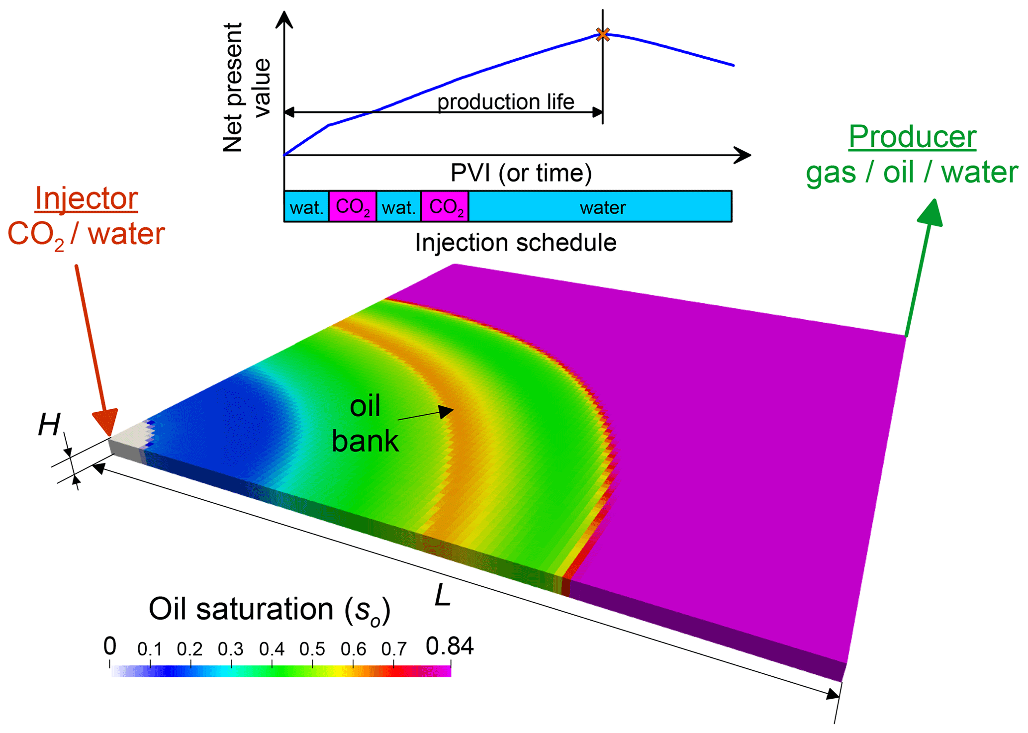
Figure 1Sketch of the areal study (a quarter of the five-spot pattern). The colour shows the distribution of oil saturation in the optimized strategy 2(WG)W at PVI=0.25, Ω=2 and the net revenue for oil exporting of ro = USD 12.5 per one barrel of oil.
Numerical modelling of CO2 flooding is often conducted by employing compositional reservoir simulations, which allow for detailed estimation of compositional exchanges between the gas and oil phases (Coats, 1980; Orr et al., 1995). This complicates the optimisation, because compositional modelling is computationally expensive. Consequently, the optimal injection strategy should be determined with a rather limited number of compositional runs. Additional efforts to accelerate the numerical optimisation should be undertaken to allow for an accurate solution to be reached within a reasonable computational time. The improvement can be achieved by either acceleration of forward simulations, e.g. by using proxy modelling (Amini and Mohaghegh, 2019; Wang et al., 2019), or implementing a modified optimisation method specially designed for such studies (Chen and Reynolds, 2016).
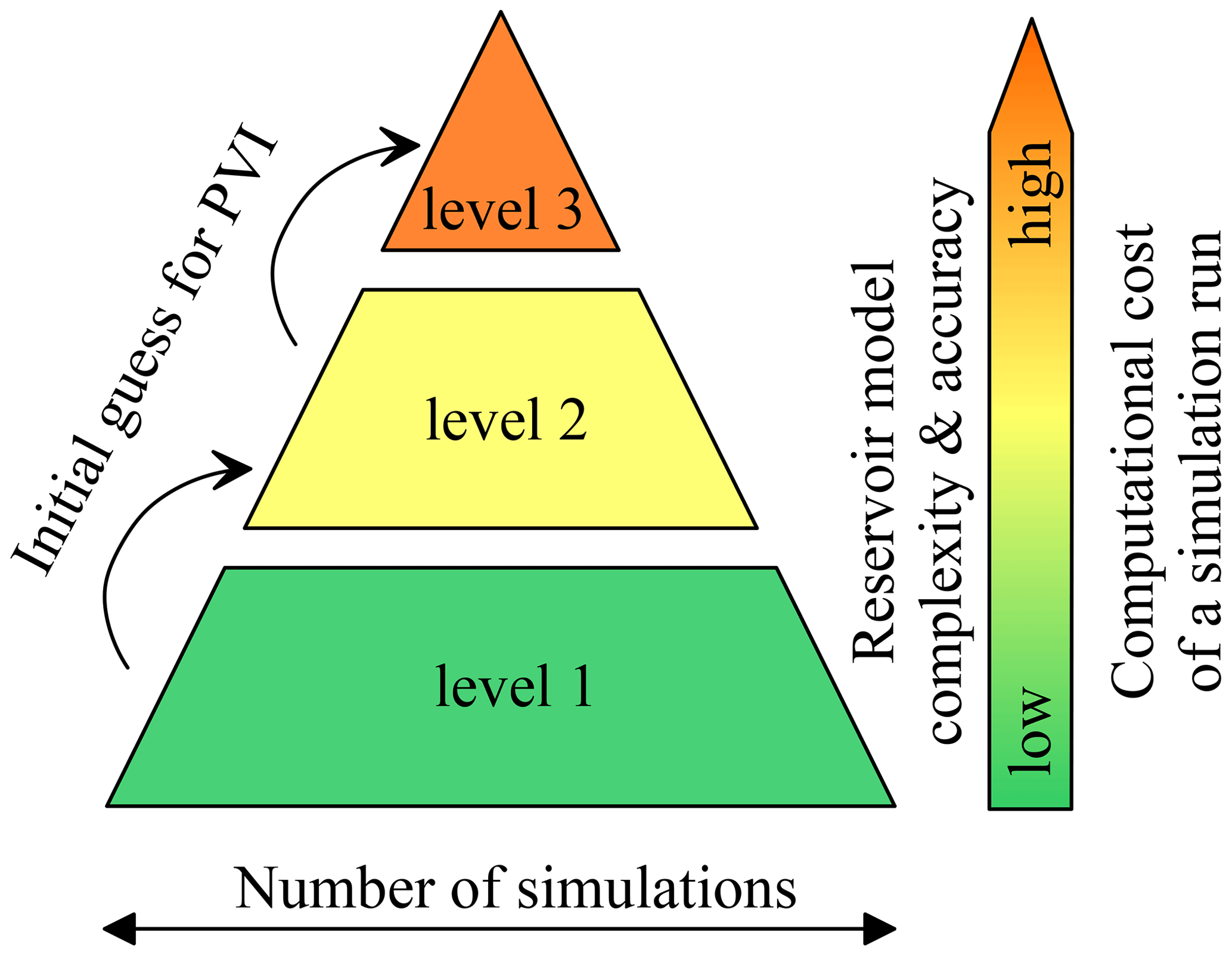
In this paper, we aim to present our approaches for the numerical optimisation of gas flooding scenarios. Here, we constrain the investigation to determining the optimal volumes of gas and oil slugs for the case of areal CO2 injection. Finding optimal well patterns and distances between injection and producing wells is beyond the scope of this work. The idea behind our approach is to construct a hierarchy of reservoir models of increasing complexity (Fig. 2). The top level corresponds to the reservoir model that needs to be optimised, whereas the lower levels correspond to coarser approximations of the top-level model. We intend to begin optimisation with the most coarse model on the first level, which allows for many computationally-cheap simulation runs. Thus, we can explore a large region of the parameter space and find a good approximation of the injection schedule near the global maximum of NPV. When going up the hierarchy, the initial guess for the optimal volumes of the water and gas slugs (i.e. pore volumes injected (PVI)) on the next level is equal to the volumes obtained on the previous level of the hierarchy. The determined PVI are then used as the initial guess on the next level, where a more refined reservoir model is employed. Since the refined model requires lager computational resources, we aim to reduce the number of simulation runs for this model. This is achieved by ensuring that the coarser model from a previous level provides a good estimate for the solution to the optimisation study on the next level.
This article is organised as follows. In Sect. 2, we describe a hierarchy of synthetic models of WAG and briefly overview all governing equations for both the fluid transport and economic processes. In Sect. 3, we discuss the objective function and its noisy behaviour at large timesteps. In Sect. 4, we present the details of the proposed optimisation method. In Sect. 5, we discuss the result of the numerical experiments related to the optimisation of different gas flooding strategies. We end the article with the conclusions in Sect. 6.
2.1 Overview of the reservoir models
For estimating NPV of CO2 flooding, we use the mathematical model presented in our previous work (Afanasyev et al., 2021). Generally, all parameters of the reservoir model (e.g. the fluid composition) and the economic calculations are equal to those in the noted paper. Here, we give only a brief overview of the involved modelling approaches emphasising several new developments.
A new feature of the present work is that we consider 2-D reservoir models corresponding to a quarter of the five-spot pattern (an injection pattern in which four injection wells are located at the corners of a square and the production well sits in the centre), in addition to the 1-D simulations corresponding to the slim-tube experiments. We use a Cartesian reservoir model of equal lateral extensions L and height H (Fig. 1). We denote the number of grid blocks along axes x and y by nx and ny. The number of grid blocks along the vertical axis z is always 1. Thus, we consider an areal study. Two wells are placed in the opposite corners of the sector, i.e. in the grid blocks (1,1) and (nx,ny). Water and CO2 are injected into the reservoir through the first well (Injector), whereas oil, water and gas are recovered through the other well (Producer). We search for the injection schedule, i.e. the optimal periods of water and CO2 injection, that maximises NPV.
Thereafter only two cases of nx and ny are possible:
-
1-D reservoir model (Fig. 3a). nx>1 and ny=1, i.e. the grid dimension is nx×1. This one-dimensional study was investigated in detail by Afanasyev et al. (2021). The flow occurs only in the direction of axis x, and all grid blocks in a sequence from the Injector to Producer are contacting the injected water and CO2. Thus, this case corresponds to 100 % efficient volumetric sweep, EV=1.
-
2-D reservoir model (Fig. 3b and c) with . This reservoir model corresponds to a quarter of the five-spot pattern with a regular rectilinear grid. The volumetric sweep is less efficient in this case because some oil near the distant corners from the wells is bypassed by the injection fluids.
Certainly, the 2-D model is more complicated than the 1-D model, because its dimension is higher. Therefore, it is not obvious how the conclusions of Afanasyev et al. (2021) for the 1-D model can be applied to this simulation setup. In part, this study concerns comparison of the optimal strategies in the 1-D and 2-D studies.
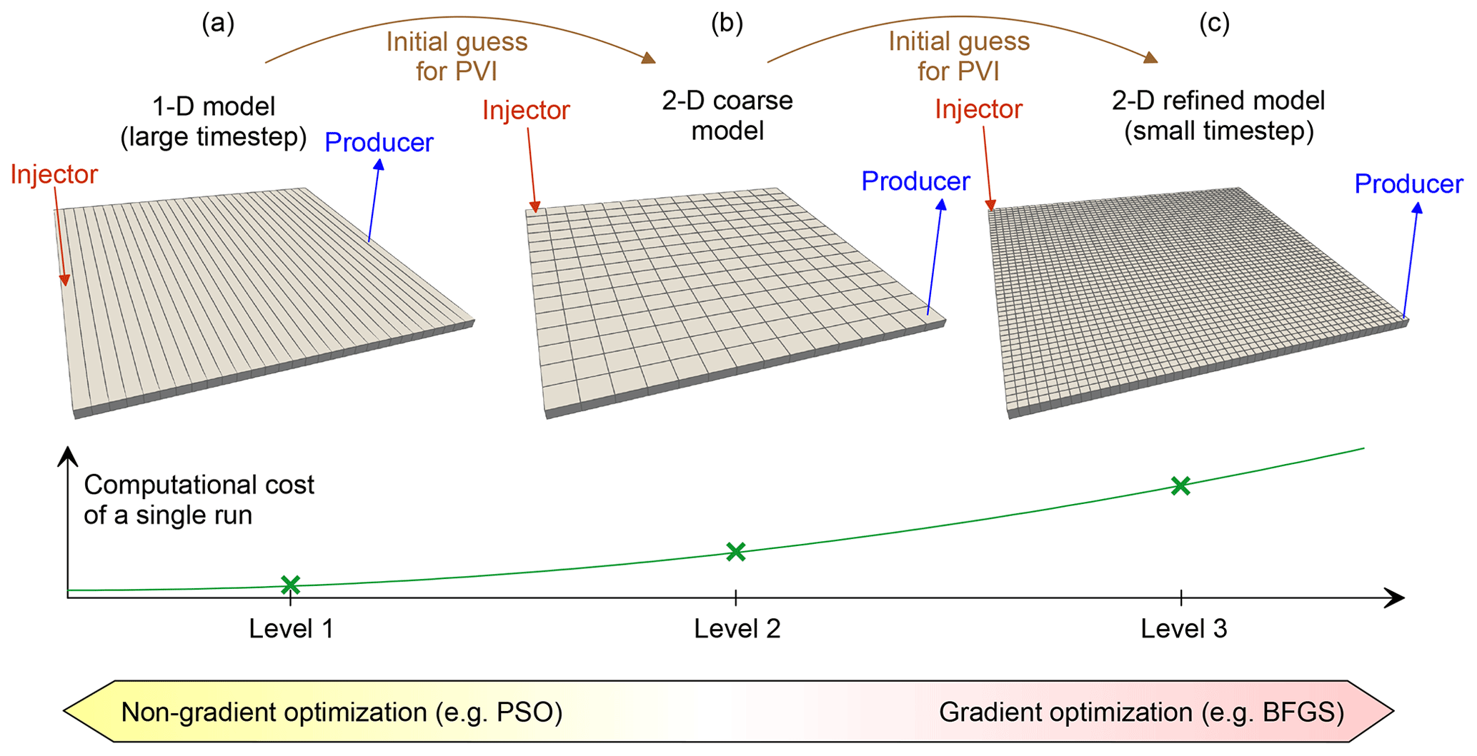
Figure 3Sketch of the proposed optimisation method. The 1-D reservoir model is shown on the left (a). The 2-D reservoir models of different grid resolution are shown on the right (b, c).
2.2 Governing equations
We employ compositional simulations to estimate the efficiency of oil recovery. We use the three-component mixture CH4–C6–C16 as a proxy for oil. The initial molar composition of fluid is 20 % CH4, 40 % C6 and 40 % C16 (Orr, 2007). The reservoir pressure is 139 bar (the minimum miscibility pressure (MMP) is ≈205 bar) and reservoir temperature is 93 ∘C. The phase equilibria are simulated using the Soave-Redlich-Kwong equation of state with volume shift (Redlich and Kwong, 1949; Soave, 1972). The viscosity of hydrocarbon phases is predicted using the LBC-correlation (Lohrenz et al., 1964). The water viscosity is 0.35 cP. The connate water saturation is swc=0.16. The residual saturation of oil is 0.24. The numerical modelling and optimisation is conducted in our MUFITS simulator (Afanasyev, 2015, 2020; Afanasyev and Vedeneeva, 2021).
We investigate immiscible gas injection because the reservoir pressure is much lower than MMP (Johns and Dindoruk, 2013). We assume that during the injection, the reservoir pressure does not significantly deviate from its initial value. This can correspond to the case of a high-permeability reservoir. Thus, the changes in pressure do not influence the phase equilibria and miscible displacement is considered in the approximation often employed in the method of characteristics (Pope, 1980; Orr et al., 1995; LaForce and Jessen, 2010). Thus, our study does not concern injection strategies implementing pressurisation to reach miscibility (Langston et al., 1988).
To estimate the economic efficiency of the injection, we couple the reservoir model with a simple model of cash flow. The economic estimates are based on the calculation of NPV, where the cash flow includes the expenses for the water injection and disposal (USD 2 and 1.5 per one barrel of oil) and CO2 injection and separation (USD 2.55 and 1.33 per one million standard cubic feet), and the net revenue ro for oil exporting, typically ro= USD 12.5 per one barrel of oil (Tzimas et al., 2005; Salem and Moawad, 2013; Rodrigues et al., 2019). These and other parameters of the coupled reservoir and economic model are identical to those in Afanasyev et al. (2021).
2.3 Dimensionless variables
The hydrocarbon pore volume, , is identical in the 1-D and 2-D models, where ϕ is the porosity. Therefore, it is convenient to compare the models by introducing dimensionless quantities that are identical in both cases (Afanasyev et al., 2021).
where PVI is the number of injected pore volumes, t is the injection time, Q is the volume injection rate (at reservoir pressure), J is the dimensional net present value, is the net revenue for exporting unit volume of reservoir oil, tds is the discount period, D is the discount rate, and Ω is the dimensionless injection rate. As shown in Afanasyev et al. (2021), the variables in Eq. (1) allow the number of parameters that the optimal injection strategy depends on to be reduced and thus, help to scale up the estimates.
2.4 Injection strategies
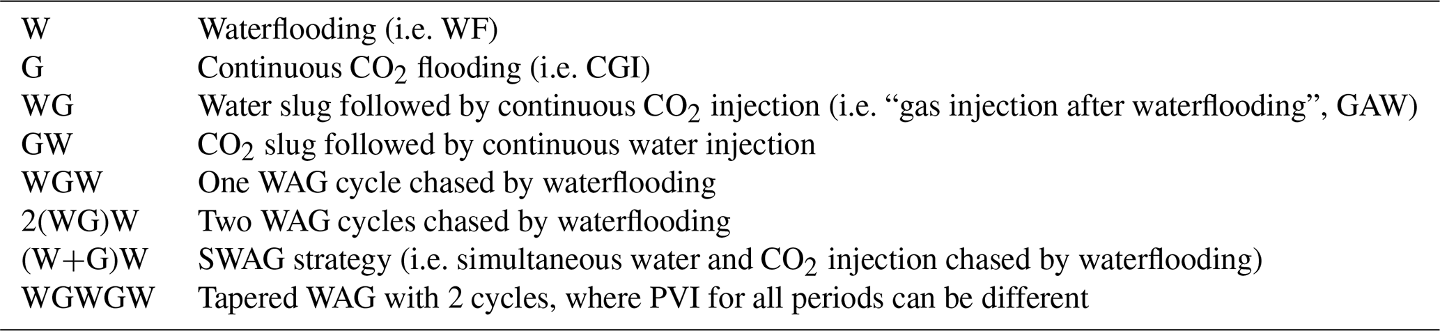
We denote the periods of water injection by the symbol W, the periods of gas injection by G, and the period of simultaneous water and gas injection by the abbreviation W+G. Each period is characterised by the number of injected pore volumes, PVIi. The periods W+G are also characterised by the volume fraction of gas in the injected fluid (at reservoir conditions). We abbreviate the strategies by a series of the noted symbols corresponding to the sequence of the injection periods in the order of increasing time. For example, the abbreviation GW denotes the strategy corresponding to CO2 injection over an initial period chased by waterflooding. The abbreviations of all strategies considered in this study are summarised in Table 1. The injection rate, Ω, is kept constant over all periods.
2.5 Optimisations criterion
For given parameters, e.g. Ω and ro, we search for the optimal parameters of the strategies given in Table 1 by using the following criterion:
Thus, the total injection volume, which can be regarded as the production life of the reservoir, is determined in the optimisation study rather than being a given quantity.
3.1 Parametrisation
Consider the case of optimising the WAG strategy 2(WG)W involving two identical WAG cycles followed by waterflooding (Table 1). This strategy is characterised by the volumes of water and gas slugs in every cycle, which we denote by PVI1 and PVI2, and the duration of the latest waterflooding, which we denote by PVI5. The cycles are identical, i.e. PVI3≡PVI1 and PVI4≡PVI2. Thus, the total volume of injected CO2 is , and the total volume of injected water in the WAG cycles is . It is assumed that the maximum of NPV (denoted by NPVopt) is reached at the end of the latest water injection period, i.e. when the total injection volume is
The parameter space for the strategy 2(WG)W is three-dimensional . We employ an optimisation method that allows acceleration to be achieved by reducing the dimension by one, and thus, the two-dimensional parameter space to be considered {PVI1,PVI2}. The method is based on the introduction of the confidence interval [0, PVImax] such that PVIopt certainly belongs to it, i.e. PVI. Based on our previous study (Afanasyev et al., 2021), we choose PVImax in the range 1.2–1.5. For a given PVI1 and PVI2, the injection is always simulated until PVImax is reached. In the numerical modelling, the simulator is forced to calculate NPV at the end of every timestep and commit to memory the current PVI and NPV, if the current NPV is larger than all values of NPV at the previous timesteps. Thus, at , the simulator can report a good estimate for PVIopt and NPVopt given that the timestep ΔPVI is small enough. Indeed, the values of PVIopt and NPVopt are those committed to the memory.
Let us explain the method in detail. The typical shape of the NPV(PVI) curve is shown in Fig. 4. With increasing PVI, NPV increases until point Aopt is reached and then decreases because the expenses exceed the revenue. Given that the timestep is constant (ΔPVI=const), the simulator determines only a countable set of points Ai, on the curve, where N is the total number of timesteps needed to reach PVImax. Assume the reservoir simulator is at the moment in time in the simulation schedule corresponding to point A1. Then, the abscissa and the ordinate of this point correspond to the current values of PVIopt and NPVopt, because the NPV(PVI) increases at A1 (Fig. 4). After another timestep, the dimensionless time increases by ΔPVI and the simulator calculates the next point A2 on the curve. Since the ordinate of A2 is larger than that of A1, the simulator replaces PVIopt and NPVopt with the coordinates of point A2. The same occurs when the simulator goes on from A2 to A3. Assume the true maximum of NPV, i.e. the true NPVopt, is reached in point Aopt between A2 and A3 as shown in Fig. 4. After the simulator performs another timestep and calculates A4, it does not change PVIopt and NPVopt, because the ordinate of A4 is less than that of A3. Thus, PVIopt and NPVopt remain the coordinates of point A3. The same occurs when the simulator goes on from A4 to A5 and further, if NPV(PVI) is a decreasing function near and to the right of A4 and A5. Therefore, the values of PVIopt and NPVopt that the simulator reports at PVImax are the coordinates of point A3.
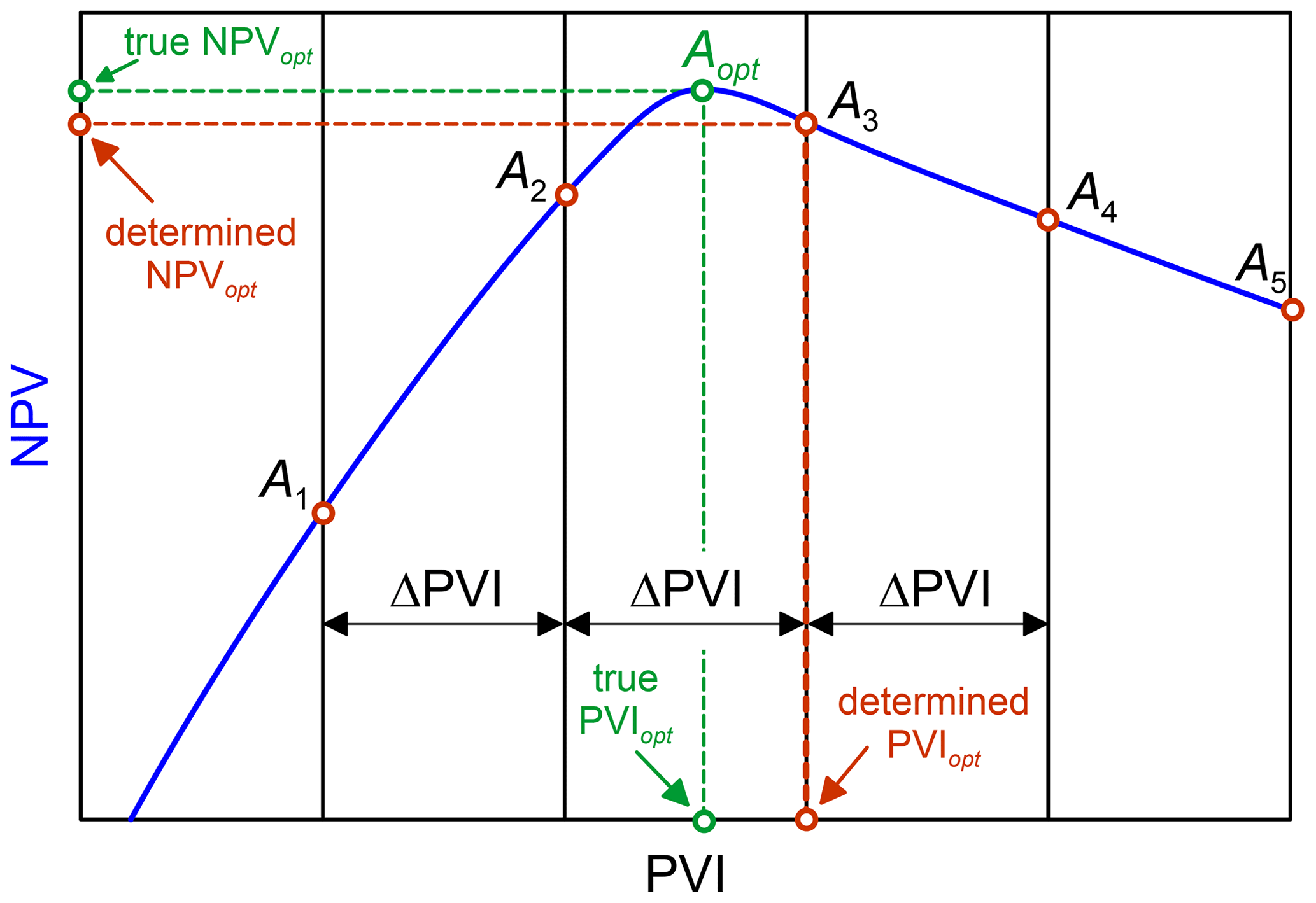
Figure 4True against determined values of PVIopt and NPVopt in the compositional simulation. The timestep is ΔPVI.
As follows from the described approach, the determined value of NPVopt is slightly less than the true NPVopt (point A3 lies below Aopt in Fig. 4). The error in the determined PVIopt and NPVopt decreases with decreasing ΔPVI as more points Ai are calculated on the curve NPV(PVI). Typically, we choose ΔPVI in the range 0.001–0.025, but the selection criteria for ΔPVI are discussed in detail in Sect. 3.4.
We can regard NPVopt and PVIopt as the functions of only two variables, PVI1 and PVI2, by implementing the described approach. According to Eq. (3), the duration of the latest waterflooding, PVI5, can be determined as
Generalising for other strategies the proposed reduction in the parameter space dimension, we can assume that the dimension is one less than the number of independent variables. For example, the dimension for the strategy WGW is 2, the dimension for WG and GW is 1, and the dimension for W and G is 0. In the latter case, it is sufficient to conduct just one simulation to determine the optimal PVIopt and NPVopt. The parameter space dimension for the (W+G)W strategy is two-dimensional because the period of simultaneous water and CO2 injection is characterised by two variables, i.e. the duration of the injection period and the gas volume fraction.
3.2 Typical shape of the objective function
The contour lines of the objective function NPVopt(PVIw,PVIg) for the strategy 2(WG)W are shown in Fig. 5. The contours are calculated at Ω=2 and ro= USD 12.5 per one barrel of oil. In both 1-D and 2-D studies, the maximum of NPVopt, i.e. NPV* (see Eq. 2) is reached at PVIw≈0.25 and PVIg≈0.28 (point O*). Thus, the volumes of water and gas slugs in the cycles are PVI1≈0.125 and PVI2≈0.14, respectively. These quantities characterise the optimal strategy 2(WG)W. However, the region of high values of NPVopt is quite large and extends into the region of high values of PVIg. This means that large NPV can also be achieved at a higher volume of CO2 injection, although the most optimal parameters are at point O*. On the contrary, if PVIg decreases and becomes less than 0.1, then NPVopt rapidly decreases. Thus, reducing the CO2 slug volume below a certain limit (i.e. PVIg≤0.1) causes a significant profitability reduction.
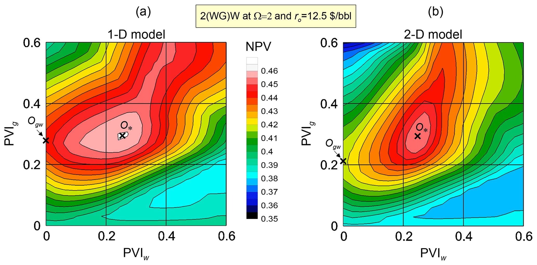
Figure 5The objective function NPVopt(PVIw,PVIg) for the strategy 2(WG)W. The functions for the 1-D and 2-D reservoir models are shown in panels (a) and (b), respectively.
In the limit PVIg=0, the duration of the periods of CO2 injection becomes 0 and the strategy 2(WG)W degenerates into W. In this case, all injection periods correspond to water injection. Only their total duration PVIopt is relevant, whereas PVI1 and PVI5 can take any values such that . Consequently, NPVopt does not depend on PVIw at PVIg=0 and the contour line NPVopt=0.384 (in the 2-D model) coincides with the straight line PVIg=0 (Fig. 5). This value NPVopt=0.384 is the maximum of NPV that can be achieved by waterflooding. Note that for 2(WG)W in the 2-D model.
At a fixed PVIg, the reduction in PVIw corresponds to smaller volumes of the water slugs. In the limit PVIg=0, the strategy 2(WG)W degenerates into GW, where two periods of CO2 injection stick together and can be regarded as a single period G. The maximum of NPVopt at PVIw=0 is reached in point Ogw (Fig. 5). This point corresponds to for the strategy GW. As follows from the contour lines in Fig. 5, the gain in NPV that can be obtained by choosing the 2(WG)W strategy instead of GW is larger for the 2-D model than for the 1-D model. Obviously, this is caused by a more significant influence of the WAG injection on the areal sweep efficiency in the 2-D case than in the 1-D case where EV is always 1.
3.3 Noisy behaviour of the objective function
The objective function NPVopt exhibits a noisy behaviour because of the time discretisation in the numerical modelling. Indeed, the accuracy of determined NPVopt is higher at smaller timesteps ΔPVI (Fig. 4). To estimate the noise introduced by the timestepping, consider the function NPVopt(PVIw,PVIg) for the strategy 2(WG)W in the vicinity of its maximum O* at PVIw≈0.25 and PVIg≈0.28 (Fig. 6). The function NPVopt is a rather smooth function over the considered range of PVI at a small timestep ΔPVI=0.001 (Fig. 6). With increasing ΔPVI, the contour lines of NPVopt become more skewed, because Aopt switches between different points Ai, shown schematically in Fig. 4. At large ΔPVI=0.025, the noise amplitude becomes so large that NPVopt exhibits several local maxima near the true maximum in point O*. Certainly, there is another source of noise in NPVopt related to the space discretisation (i.e. the grid resolution). But thereafter, we assume that the influence of ΔPVI is dominant, which is supported by the numerical experiments.

Figure 6The objective function NPVopt calculated using the 2-D model for different values of ΔPVI = 0.001 (a), 0.005 (b), and 0.025 (c). The lower panels show the slice of NPVopt at PVIg=0.29.
The noisy behaviour poses additional difficulties for the numerical optimisation, which can exhibit poor convergence. Thus, the reduction of the noise amplitude is relevant. As shown above, the noise can be reduced by using smaller timesteps ΔPVI. However, this can be done at the cost of more computationally expensive simulations (Fig. 7). Indeed, for a fixed PVImax, a smaller ΔPVI forces the reservoir simulator to perform a larger number of timesteps that can be estimated as . Assuming that all timesteps require an equal number of linear and non-linear iterations and flash calculations (Michelsen, 1982), an order of magnitude reduction in ΔPVI approximately results in an order of magnitude increase in the computational cost of a single compositional run. A good optimisation should balance between accuracy and computational cost by using compositional simulations with different ΔPVI and grid resolution nx.
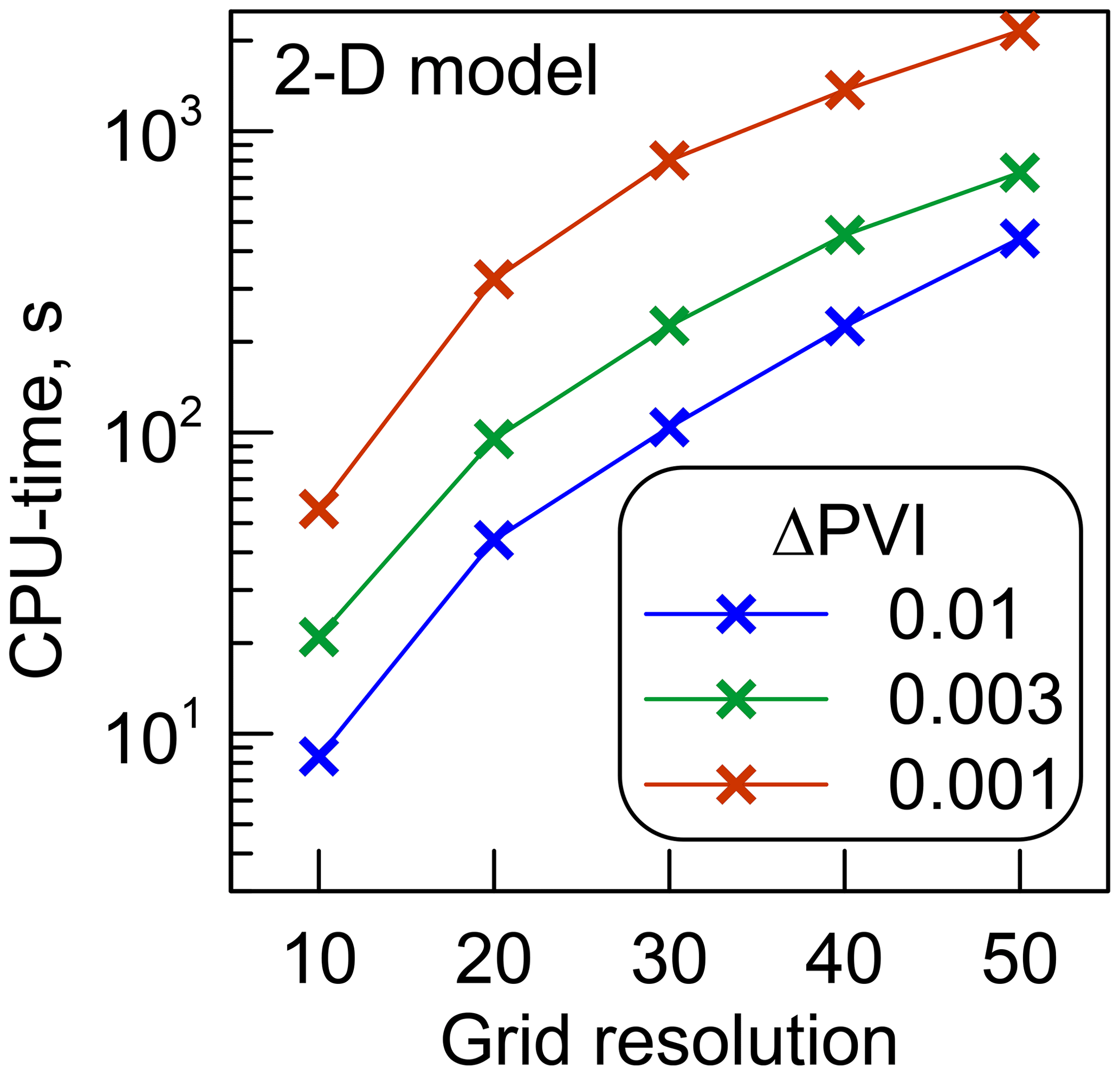
Figure 7Typical simulation time for the 2-D model against the grid resolution (nx=ny) for different timesteps ΔPVI.
3.4 Gradient against non-gradient algorithms
The noted behaviour of the objective function requires careful selection of the optimisation algorithms. Certainly, if ΔPVI and, thus, the noise amplitude are large, then the optimisation algorithms based on the calculation of the NPVopt gradient cannot be applied. Indeed, as shown in Fig. 6, the local gradient can point away from the direction of the global maximum, causing a poor convergence (Fletcher, 2000). When using the gradient algorithms, it is important to carefully choose the step quantity in the numerical differentiation, δPVI. The derivative of the objective function can be approximated as:
where PVI denotes one of the variables that NPVopt depends on. A larger δPVI can override the noise, but it also results in a poor convergence near the maximum of NPVopt. A general rule that we follow is that the gradient algorithms are applied if ΔPVI≤δPVI, where δPVI = 0.0025 is considered fixed in this study.
At large ΔPVI, the non-gradient (e.g. stochastic) optimisation algorithms are more preferable. In such cases, the compositional simulations are less computationally expensive (Fig. 7) and thus, more simulation runs can be done with the same computational resources. This is advantageous for the stochastic algorithms that normally require a larger number of iterations than the gradient algorithms.
4.1 The hierarchy of reservoir models
We propose a hybrid optimisation method based on the construction of reservoir models of increasing complexity and the implementation of both stochastic and deterministic algorithms (Figs. 2 and 3). The top level of the hierarchy corresponds to the reservoir model that needs to be optimised. It can be a 2-D or 3-D model, possibly with a fine grid. We assume that such a detailed compositional model is computationally expensive and should not be simulated too many times. Going down from the top (e.g. Level 3 in Fig. 3) to the bottom levels of the hierarchy, the number of grid blocks reduces as the model becomes coarser. For example, a coarser grid can be applied (Level 2) or even the dimension of the study can be reduced (Level 1). At lower levels, the models can also employ larger timesteps, ΔPVI, being coarser in terms of the time truncation error. Thus, more iterations of the optimisation algorithm can be carried out at the lower levels with the given computational resources.
An important property of the hierarchy is a good scaling of the solution to the optimisation study. The optimal volumes of the water and gas slugs, PVIi, determined with the models at a current level must provide a good approximation to the solution at the next level up. Thus, the initial guess for PVIi can be transferred up the hierarchy (Fig. 2). Therefore, the models of the lower levels, because they are less computationally expensive, are employed for estimating PVIi used as the initial guess in the upper levels.
Thus, the method includes finding the solution to the optimisation problem at a lower level. Then, the determined solution is passed to the next upper level where it is used as the initial guess for PVI. Then, the optimisation problem is solved at this upper level. This sequence of steps is repeated until the uppermost level of the hierarchy is reached. Since the lower levels are used only for constructing the initial guess, the solution to the optimisation problem at all levels except the uppermost level may be inaccurate. Therefore, a large timestep, e.g. ΔPVI≥0.01, is recommended at the lowest levels to make the compositional simulations even cheaper. As discussed in Sects. 3.3 and 3.4, this results in a noisy behaviour of NPVopt and requires application of a non-gradient optimisation algorithm at the lowest levels. For example, the particle swarm optimisation (PSO) can be employed to search over a large region of the parameter space for a good approximation of the global maximum of NPVopt (Kennedy and Eberhart, 2021). This is a useful property of the method, because NPVopt can exhibit several local maxima (Afanasyev et al., 2021). Using a stochastic optimisation, which usually requires a larger number of iterations than in a gradient optimisation, is reasonable on the lowest levels, where the compositional simulations are cheap (Fig. 3). Moreover, the stochastic optimisation is recommended for the lowest levels to determine a good approximation of the global maximum of NPVopt.
At the upper levels of the hierarchy, a gradient algorithm of optimisation, e.g. the Broyden–Fletcher–Goldfarb–Shanno algorithm (BFGS; Broyden, 1970), is more preferable (Fig. 3). This is justified since the gradient optimisation usually requires fewer iterations and the simulations get more expensive up the hierarchy. Moreover, the upper levels do not require a large number of simulations to explore the whole parameter space. Since an approximate location of the global maximum is known from the lowest Level 1, the volumes PVIi change only locally near the global maximum.
4.2 1-D versus 2-D simulations
The proposed method is rather straightforward. However, its successful implementation is based on the assumption that the solution at every given level provides a good initial guess for the next upper level. This assumption is not questioned in the case of simply increasing the grid resolution (e.g. the transition from Level 2 to Level 3 in Fig. 3). However, if the reservoir model changes more significantly, e.g. the problem dimension changes (the transition from Level 1 to Level 2 in Fig. 3), then the validity of this assumption is not obvious. It should be validated in every particular case and a good parametrisation of the hierarchy is the recipe for success.
Consider a particular case of the parametrisation introduced in Sect. 3.1. Its implementation for optimising the 2-D areal gas flooding is based on the assumption that the solution to the 1-D optimisation study is a good approximation of the solution to the 2-D study. This implies that the optimal dimensionless volumes of the water and gas slugs are close in the 1-D and 2-D models. The validity of such an assumption is not obvious given that EV=1 for the 1-D study and the areal (i.e. volumetric) sweep efficiency can potentially be rather small for the 2-D study due to the viscous instability and channelling. Further, we prove that it is pretty accurate over a large region of the parameter space and for various injection strategies if criterion Eq. (2) is used in the optimisation.
As shown in Fig. 8, the objective function NPVopt(PVI1) and the total injection volume PVIopt(PVI1) for the strategies WG and GW are close in the 1-D and 2-D models. The optimal PVI1 of the first water and gas slug, respectively, PVI* and NPV* in the 1-D problem, are close to those in the 2-D problem. The corresponding functions NPVopt look somewhat similar, although NPVopt in the 2-D case is smaller than in the 1-D case, particularly at PVI1=0 due to lower areal sweep efficiency. However, the global maximum of NPVopt is approximately at the same PVI1 in both cases. Thus, the solution to the 1-D study serves as a good approximation of the solution to the 2-D study for the considered Ω, ro and injection schedules. A similar behaviour shows the 2(WG)W strategy (Fig. 5).
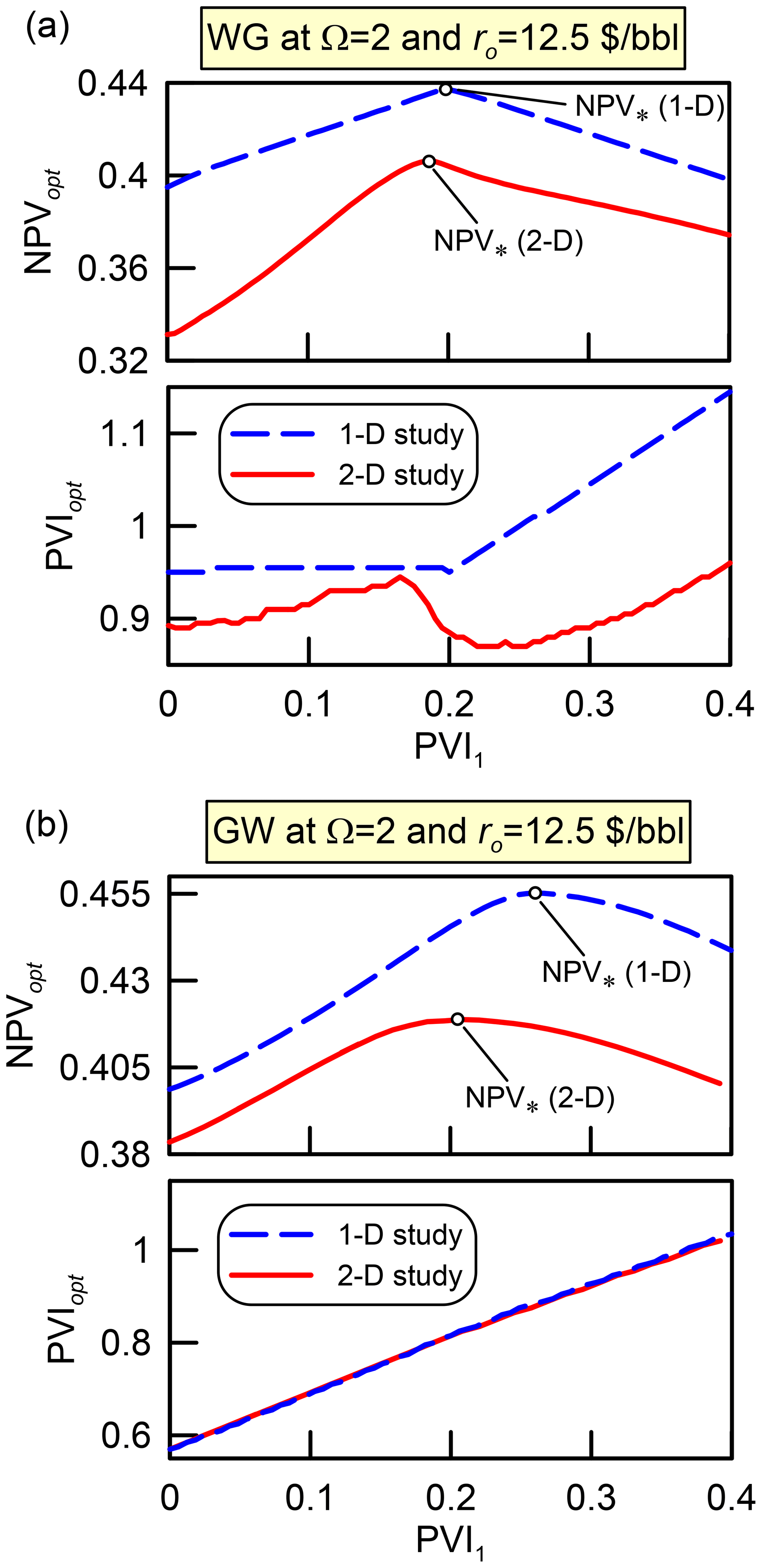
Figure 8The objective function NPVopt and the production life PVIopt for the 1-D and 2-D simulations of the strategies WG and GW at Ω=2 (panels a and b, respectively).
The results of other numerical experiments are summarised in Fig. 9. In the cross-plot, the abscissa and the ordinate of every point correspond to the same and independently optimised strategies using the 1-D and 2-D models, respectively. All parameters characterising each strategy, i.e. PVIi for all injection periods and the gas volume fraction for the simultaneous injection W+G (sg), are plotted along the axes. The maximum injection rate and the net revenue are varied in the range and ro= USD [12.5,25] per one barrel of oil. All calculated points group near the dashed straight line, ensuring that the optimal solutions for both 1-D and 2-D studies are close. Thus, the optimised strategies in the 1-D case serve as a good approximation of the optimised strategies in the 2-D case.
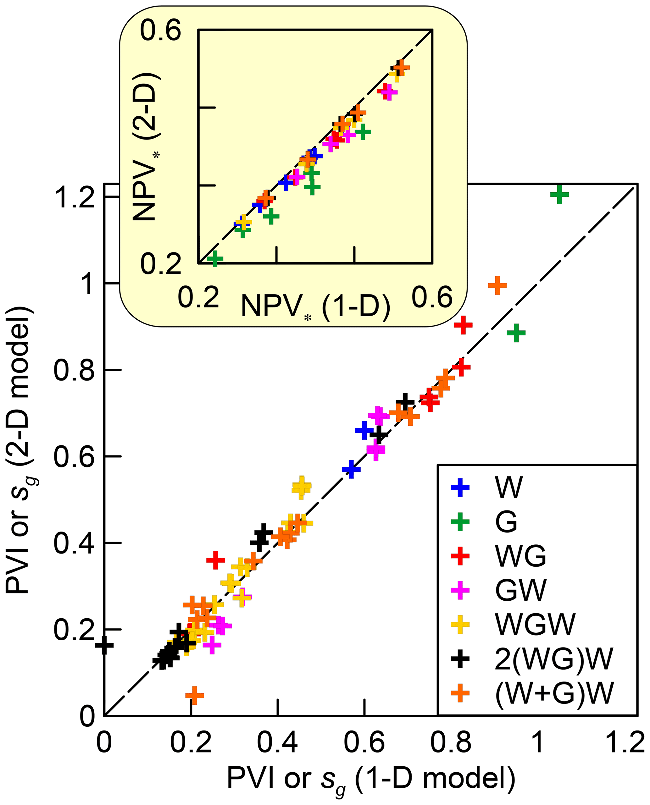
In all cases, the quantity of NPV* in the 2-D models is slightly less than in the 1-D models (Fig. 9). This is caused by a less efficient areal sweep in the 2-D models. Since the injected fluids do not contact the most distant areas from the wells, the oil recovery efficiency and, thus, NPV* are smaller.
5.1 Overview
The results of the CO2 flooding optimisation with the proposed method are summarised in Figs. 10 and 11. The injection schedules determined on each level of the hierarchy are shown with the horizontal bars, where the durations of the injection periods in PVI are given within the rectangles. The total width of the bars shows the bulk injection volume at the moment in time when the maximum of NPV is reached (i.e. at PVIopt). The optimisation algorithm, the grid resolution and the timestep used on each level are noted above the corresponding bar. The movement up the hierarchy corresponds to the movement from top to bottom in the diagrams. The changes in NPV as the optimisation progresses up are shown in the right-hand panels of the diagrams. The uppermost NPV is the net present value determined on the lowest level of the hierarchy. When the algorithm moves to the next level, first it recalculates NPVopt using the reservoir model of the next level and the injection schedule of the previous level. This NPVopt is the upper of the two quantities shown to the right of the corresponding bar. It can be slightly smaller than that determined on the previous level due to changes in the grid resolution and the dimension of the study. Then, the optimisation is conducted on the next level and NPV increases up to the lower value shown to the right of the bar. The lowest number in the right column is NPV* in the optimised strategy, i.e. NPV determined on the uppermost level of the hierarchy.
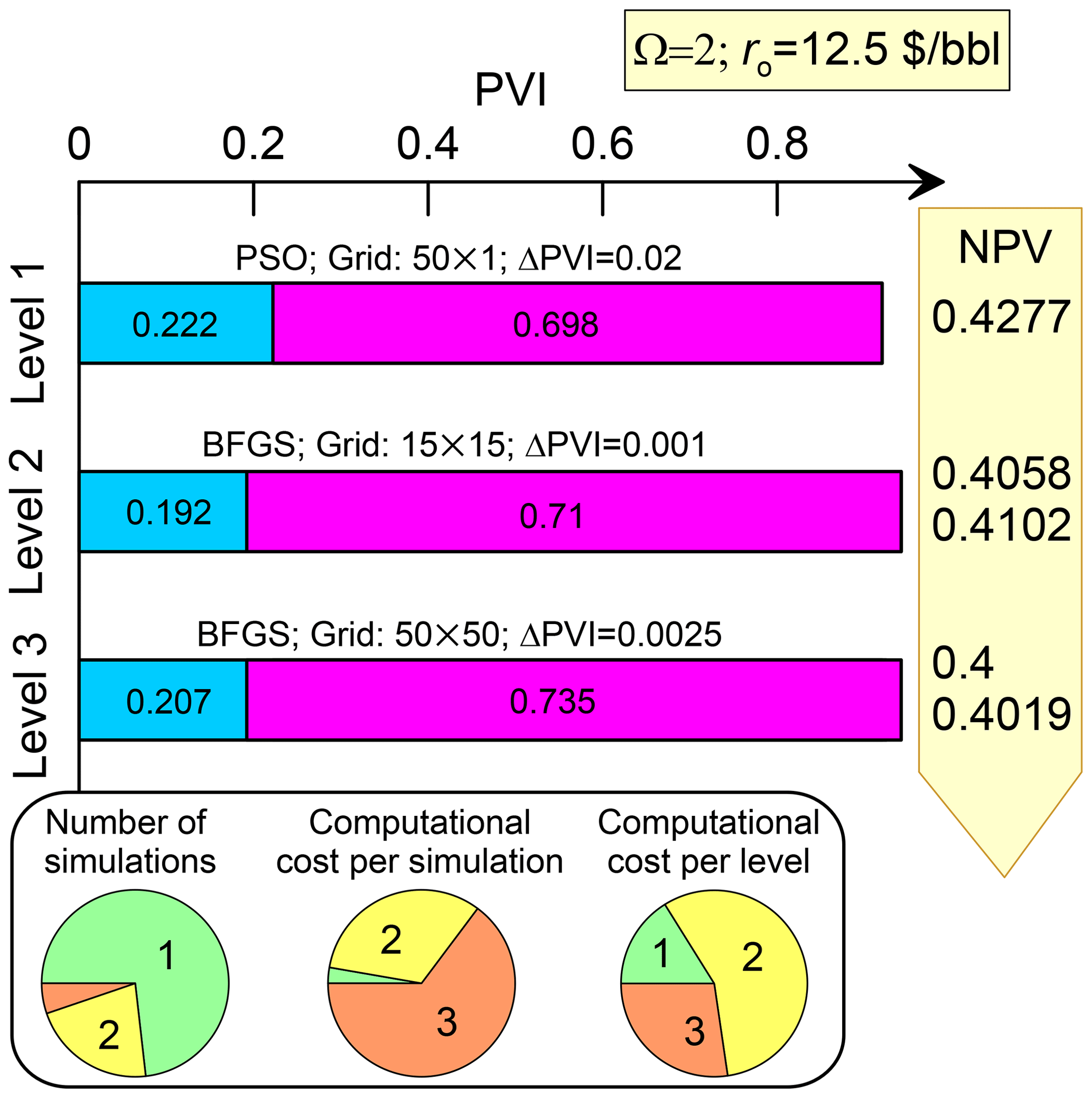
The bottom panel in each diagram shows the distribution of the computational resources between the levels (Figs. 10 and 11). From left to right, the circle charts indicate the number of compositional simulations on each level, the computational cost per simulation and the computational cost per level.
For argument's sake, we assume that even approximate values of the slug volumes are unknown before the optimisation, although they can be estimated from our previous work (Afanasyev et al., 2021). Thus, we suppose that even an approximate solution to the 2-D study is unknown and the optimisation begins from scratch. Our only assumption is that the confidence interval for the optimal slug volumes is , which is not very restrictive. Further, we discuss the algorithm performance for three different strategies of increasing complexity.
5.2 The WG strategy optimisation
The results of the hierarchy of models application for the WG strategy optimisation are summarised in Fig. 10. We apply the PSO algorithm on the lowest level. The number of particles is set equal to 16. They can move 7 times, thus 112 compositional simulations are conducted on the lowest level. In this and any other implementation of PSO, the inertia weight is 0.5 and the acceleration coefficients to the best location of both a particle and the swarm are 2.0. Due to the reasons discussed in Sect. 4, we employ a rather coarse 1-D study on the lowest level (Fig. 3). Each simulation involves only 50 grid blocks and the timestep is very large, ΔPVI=0.02, resulting in a very low computational cost per simulation on Level 1. Consequently, Level 1 acquires less than of the total computational resources for the optimisation study, even though almost of the compositional simulations are conducted on this level.
On Level 2, we switch to the coarse 2-D model and employ the BFGS algorithm, i.e. the gradient optimisation. This requires a smaller timestep, ΔPVI=0.001, to make the objective function smooth. Consequently, the computational cost per simulation is much larger on Level 2 than on Level 1, even though the number of grid blocks does not increase significantly (from 50 to 225). This is caused by a 20 times larger number of timesteps that the simulator is forced to perform on Level 2. As a result, Level 2 is the most time-consuming step of the optimisation.
On Level 3, we switch to the fine 2-D model involving 50 grid blocks along both axes, i.e. 2500 grid blocks in total (Fig. 3). In an attempt to reduce the computational cost, we specify a less restrictive constraint on the timestep, ΔPVI=0.0025, than on Level 2. Nevertheless, a compositional simulation on Level 3 takes twice as many computational resources. We assume that ΔPVI=0.0025 still is a reasonable timestep to converge to a point near the global maximum of NPVopt. Due to a smaller number of simulations, Level 3 appears to be less expensive than Level 2.
The volumes of the water and gas slugs do not significantly change up the hierarchy (Fig. 10). For instance, PVI1 is 0.222 on Level 1, then it is changed to 0.192 and finally, to 0.207 on Level 3. Again, this supports that the optimised injection schedules for the 1-D and 2-D models are pretty similar. At the same time, NPV* reduces considerably from 0.4277 to 0.4019, reflecting that EV<1 in the 2-D model.
5.3 The WAG strategies optimisation
Now we discuss the method performance in the case of the strategy 2(WG)W (Fig. 11a and b). We apply the same sequence of algorithms as in the case of the strategy WG, i.e. PSO on Level 1 and BFGS on Levels 2 and 3. Only insignificant changes of the slug volumes occur when moving up the hierarchy. Similarly to the strategy WG, the method involves a larger number of cheap compositional simulations on Level 1 and a smaller number of expensive simulations with the fine reservoir model on Level 3.
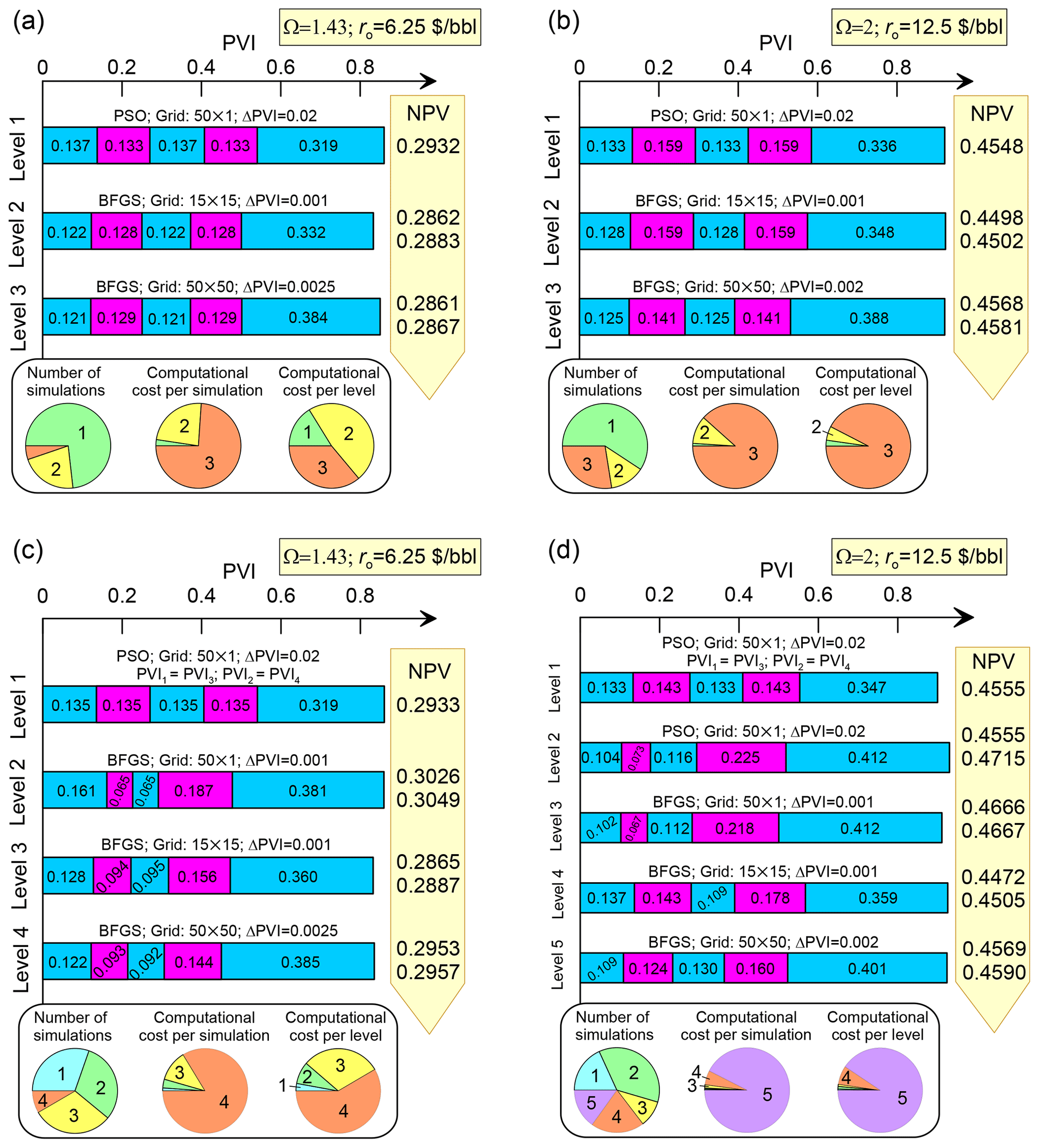
Figure 11Diagrams showing the method performance in the 2(WG)W (a, b) and WGWGW (c, d) strategies optimisation. The results are for Ω=1.43 and ro= USD 6.25 per one barrel of oil in panels (a) and (c) and Ω=2 and ro= USD 12.5 per one barrel of oil in panels (b) and (d).
Actually, the method performance depends on the injection rate Ω and the net revenue ro. At Ω=1.43 and ro= USD 6.25 per one barrel of oil, the optimised injection schedules are almost identical for the cases of 15×15 and 50×50 grids (Fig. 11a). Consequently, on Level 3, the BFGS algorithm needs only one iteration to converge. On the contrary, at Ω=2 and ro= USD 12.5 per one barrel of oil, the optimal CO2 slugs on Level 3 are smaller than those on Level 2 (Fig. 11b). Therefore, the BFGS algorithm requires three iterations to converge and, thus, larger computational resources on Level 3.
Consider a more complicated case of the WAG strategy with two different WAG cycles. Previously, we assumed that the slug volumes of water and gas are identical in the first and second cycles, respectively (i.e. PVI1≡PVI3 and PVI2≡PVI4). Now, this assumption is not employed, and the slug volumes can be different in the cycles. To distinguish this scenario from 2(WG)W, we denote such a strategy by the abbreviation WGWGW (Table 1). Every period of either gas or water injection has a different length. Thus, the parameter space of the strategy is four-dimensional, which corresponds to the four periods in the cycles PVIi, .
The method performance in the WGWGW strategy optimisation is summarised in the diagrams in Fig. 11c and d. Here, we introduce additional levels of the hierarchy to address the larger dimension of the study. Again, we apply the PSO algorithm on Level 1, where we assume that the WAG cycles are still identical, i.e. PVI1≡PVI3 and PVI2≡PVI4. Thus, Level 1 does not differ from that in the 2(WG)W strategy optimisation. We use this level to calculate an initial approximation of PVIi, supposing that they differ insignificantly in the two cycles.
On further levels, we allow PVI to be different, i.e. PVI1≠PVI3 and PVI2≠PVI4. In the case Ω=1.43 and ro= USD 6.25 per one barrel of oil, we optimise the 1-D model using the BFGS algorithm on Level 2. As a result, the PVI2 and PVI3 decreased significantly at the cost of the increase of PVI1 and PVI4. Then, on Levels 3 and 4, we switch to the 2-D model, first considering a coarser and then a finer grid. The noted behaviour of PVI2 and PVI3, which is first observed on Level 2, is preserved in the subsequent levels. The optimal strategy begins with the injection of a larger water slug followed by a bit smaller CO2 and water slugs. Then, the injection is followed by a large CO2 slug chased by the final waterflooding.
In the case of Ω=2 and ro= USD 12.5 per one barrel of oil, we employ PSO on Levels 1 and 2 (Fig. 11d). After Level 1, which is similar to that in the previous case, we allow the cycles to be different on Level 2 and vary in the range , where are the slug volumes determined on Level 1. The additional level allows a larger region of the four-dimensional parameter space to be explored and ensures convergence to the global maximum of NPV. Further, Levels 3–5 in Fig. 11d are identical to Levels 2–4 in Fig. 11c. Both optimisations of the WGWGW strategy require most of the computational resources on the uppermost level. It would seem that, respectively, the intermediate Levels 2 and 3 and 2–4 in Fig. 11c and d are extra levels, which can be omitted by employing the uppermost level with the 50×50 grid immediately after Level 1. However, this may lead to convergence to the local maximum at PVI1≈PVI3 and PVI2≈PVI4. Thus, the intermediate levels are relevant.
As shown in Fig. 11, the tapered WAG allows NPV to be increased by ≈0.01 and ≈0.001 at ro= USD 6.25 and 12.5 per one barrel of oil, respectively, as compared to the 2(WG)W strategy. The improvement is insignificant at least at ro= USD 12.5 per one barrel of oil. The general trend that we observe for the presented and other optimised schedules is that the gas-to-water ratio should increase with the cycle number.
Our key findings related to the optimisation of enhanced oil recovery are
-
The volumes of optimal CO2 slugs are similar in 1-D and 2-D areal displacements
-
1-D compositional simulations are efficient for optimising areal CO2 flooding patterns
Indeed, the successful implementation of the proposed method is based on the observation that the optimised injection strategies parameterised in the proposed dimensionless variables are quite similar in the 1-D and 2-D models. Although NPV* in the 2-D case is generally lower than in the 1-D case, it is achieved at approximately the same volumes of water and gas slugs (Fig. 9). This means that the conclusions of our previous study (Afanasyev et al., 2021) are applicable not only to the 1-D reservoir models corresponding to the slim-tube experiments, but also to the 2-D models corresponding to the 5-spot patterns. Therefore, it is efficient to determine the optimised strategies by using 1-D simulations, because the optimal PVI in the 1-D and 2-D cases are close to each other. Since the influence of geological uncertainties on the optimised PVI can be comparable to the PVI changes when the coarse 1-D model is replaced by the fine 2-D model, the PVI values determined with the 1-D model can be regarded as sufficiently accurate. Their changes associated with the transition to the upper levels of the hierarchy can be overridden by the geological and other uncertainties. Thus, in the field applications, the WAG process optimisation using the 1-D compositional simulations might be worth considering, if it is guaranteed that the solution to the 1-D model allows for a reasonably accurate scaling up to the 3-D flows in the reservoir. Certainly, this conclusion implies that the reservoir is rather thin and homogeneous. The reservoir heterogeneity, the gravity override and other processes can undermine the noted conclusion. Every reservoir is unique and thus, the validity of the conclusion should be judged in each case on its own merits. Here, we only argue that the conclusion is valid for the considered 2-D sector model.
An outcome of this work that is also worth mentioning is that the independent parametrisation of each WAG cycle does not result in a considerable increase in NPV*. As shown in Sect. 5.3, PVI independently determined for each cycle can be quite different in the two considered cycles. However, the corresponding increase in NPV* as compared to the case of identical WAG cycles is less than 1 %. Such behaviour indicates that the tapered WAG does not considerably improve NPV* in the considered case and if criterion Eq. (2) is employed in the optimisation. However, this is just an estimate and a subject of future research.
As we have shown, the proposed hybrid optimisation method allows the number of compositional simulations to be reduced with a fine reservoir model. A smaller number of such simulations are carried out only at the upper optimisation levels. Most of the other simulations at the lower levels are less computationally expensive. This results in significant acceleration of the numerical optimisation. Another advantage is the use of PSO at the lowest level, which ensures convergence to the global maximum of NPVopt. Certainly, the optimisation can be accelerated even further using a priori knowledge on the solution and the shape of the objective function. For example, for the considered oil composition and the reservoir pressure and temperature, any optimised WAG strategy that ends with waterflooding requires injection of PVIg≈0.3 pore volumes of CO2 (see also Afanasyev et al., 2021). This volume distribution between different WAG cycles only slightly changes NPV. Thus, PVIg=0.3 can be adopted as a good approximation for the total injected volume of CO2 instead of its estimation at the lowest levels of the hierarchy.
The executable of the MUFITS simulator used for modelling the CO2 flooding is available at http://www.mufits.imec.msu.ru/ (Afanasyev, 2021).
AAf contributed to the study conceptualisation, the methodology development and writing original draft of the manuscript. AAn and AC contributed to the numerical analysis by running MUFITS and post-processing the simulation results.
The contact author has declared that neither they nor their co-authors have any competing interests.
Publisher’s note: Copernicus Publications remains neutral with regard to jurisdictional claims in published maps and institutional affiliations.
This article is part of the special issue “European Geosciences Union General Assembly 2021, EGU Division Energy, Resources & Environment (ERE)”. It is a result of the EGU General Assembly 2021, 19–30 April 2021.
This research has been supported by the Russian Science Foundation (grant no. 19-71-10051).
This paper was edited by Christopher Juhlin and reviewed by two anonymous referees.
Afanasyev, A.: Hydrodynamic Modelling of Petroleum Reservoirs using Simulator MUFITS, Energy Proced., 76, 427–435, https://doi.org/10.1016/j.egypro.2015.07.861, 2015. a
Afanasyev, A.: Compositional Modelling of Petroleum Reservoirs and Subsurface CO2 Storage with the MUFITS Simulator, 2020, 1–13, https://doi.org/10.3997/2214-4609.202035190, 2020. a
Afanasyev, A.: MUFITS reservoir simulation software, MUFITS [software], available at: http://www.mufits.imec.msu.ru/, last access: 13 September 2021. a
Afanasyev, A. and Vedeneeva, E.: Compositional modeling of multicomponent gas injection into saline aquifers with the MUFITS simulator, J. Nat. Gas Sci. Eng., 84, 103988, https://doi.org/10.1016/j.jngse.2021.103988, 2021. a
Afanasyev, A., Andreeva, A., and Chernova, A.: Influence of oil field production life on optimal CO2 flooding strategies : Insight from the microscopic displacement efficiency, J. Petrol. Sci. Eng., 205, 108803, https://doi.org/10.1016/j.petrol.2021.108803, 2021. a, b, c, d, e, f, g, h, i, j, k, l
Amini, S. and Mohaghegh, S.: Application of machine learning and artificial intelligence in proxy modeling for fluid flow in porous media, Fluids, 4, 126, https://doi.org/10.3390/fluids4030126, 2019. a
Blunt, M., Fayers, F., and Orr, F. M.: Carbon dioxide in enhanced oil recovery, Energ. Convers. Manage., 34, 1197–1204, https://doi.org/10.1016/0196-8904(93)90069-M, 1993. a
Broyden, C. G.: The convergence of a class of double-rank minimization algorithms 1. General considerations, IMA J. Appl. Math., 6, 76–90, https://doi.org/10.1093/imamat/6.1.76, 1970. a
Chen, B. and Pawar, R.: Capacity assessment of CO2 storage and enhanced oil recovery in residual oil zones, in: Proceedings – SPE Annual Technical Conference and Exhibition, Dallas, Texas, USA, September 2018, https://doi.org/10.2118/191604-ms, 2018. a
Chen, B. and Reynolds, A. C.: Ensemble-Based Optimization of the Water-Alternating-Gas-Injection Process, SPE Journal, 21, 0786–0798, https://doi.org/10.2118/173217-PA, 2016. a
Christensen, J., Stenby, E., and Skauge, A.: Review of WAG Field Experience, SPE Reserv. Eval. Eng., 4, 97–106, https://doi.org/10.2118/71203-PA, 2001. a
Coats, K. H.: An Equation of State Compositional Model, Soc. Petrol. Eng. J., 20, 363–376, https://doi.org/10.2118/8284-PA, 1980. a
Ettehadtavakkol, A., Lake, L. W., and Bryant, S. L.: CO2-EOR and storage design optimization, Int. J. Greenh. Gas Con., 25, 79–92, https://doi.org/10.1016/j.ijggc.2014.04.006, 2014. a
Fletcher, R.: Practical Methods of Optimization, John Wiley & Sons, Ltd, Chichester, West Sussex England, https://doi.org/10.1002/9781118723203, 2000. a
Ghedan, S. G.: Global Laboratory Experience of CO2-EOR Flooding, in: SPE/EAGE Reservoir Characterization and Simulation Conference, Abu Dhabi, UAE, October 2009, Society of Petroleum Engineers, https://doi.org/10.2118/125581-MS, 2009. a
Jensen, T. B., Little, L. D., Melvin, J. D., Reinbold, E. W., Jamieson, D. P., and Shi, W.: Kuparuk River Unit Field – The First 30 Years, in: SPE Annual Technical Conference and Exhibition, San Antonio, Texas, USA, October 2012, Society of Petroleum Engineers, https://doi.org/10.2118/160127-MS, 2012. a
Johns, R. T. and Dindoruk, B.: Gas Flooding, in: Enhanced Oil Recovery Field Case Studies, Elsevier, pp. 1–22, ISBN 978-0-1238-6545-8, https://doi.org/10.1016/B978-0-12-386545-8.00001-4, 2013. a, b
Kennedy, J. and Eberhart, R.: Particle swarm optimization, in: Proceedings of ICNN'95 – International Conference on Neural Networks, vol. 4, pp. 1942–1948, IEEE, https://doi.org/10.1109/ICNN.1995.488968, 2021. a
Kovscek, A. and Cakici, M.: Geologic storage of carbon dioxide and enhanced oil recovery. II. Cooptimization of storage and recovery, Energ. Convers. Manage., 46, 1941–1956, https://doi.org/10.1016/j.enconman.2004.09.009, 2005. a
LaForce, T. and Jessen, K.: Analytical and numerical investigation of multicomponent multiphase WAG displacements, Computat. Geosci., 14, 745–754, https://doi.org/10.1007/s10596-010-9185-3, 2010. a
Lake, L. W.: Enhanced Oil Recovery, Prentice Hall, Englewood Cliffs, 550, ISBN 0-13-281601-6, 1989. a
Langston, M., Hoadley, S., and Young, D.: Definitive CO2 Flooding Response in the SACROC Unit, in: Proceedings of SPE Enhanced Oil Recovery Symposium, Tulsa, Oklahoma, April 1988, Society of Petroleum Engineers, https://doi.org/10.2523/17321-MS, 1988. a
Lohrenz, J., Bray, B. G., and Clark, C. R.: Calculating Viscosities of Reservoir Fluids From Their Compositions, J. Petrol. Technol., 16, 1171–1176, https://doi.org/10.2118/915-PA, 1964. a
Michelsen, M. L.: The isothermal flash problem. Part II. Phase-split calculation, Fluid Phase Equilibr., 9, 21–40, https://doi.org/10.1016/0378-3812(82)85002-4, 1982. a
Orr, F. M.: Theory of gas injection processes, Tie-Line Publications, Copenhagen, 2007. a
Orr, F. M., Dindoruk, B., and Johns, R. T.: Theory of Multicomponent Gas/Oil Displacements, Ind. Eng. Chem. Res., 34, 2661–2669, https://doi.org/10.1021/ie00047a015, 1995. a, b
Pope, G. A.: The Application of Fractional Flow Theory to Enhanced Oil Recovery, Soc. Petrol. Eng. J., 20, 191–205, https://doi.org/10.2118/7660-PA, 1980. a
Pritchard, D. and Nieman, R.: Improving Oil Recovery Through WAG Cycle Optimization in a Gravity-Overide-Dominated Miscible Flood, in: SPE/DOE Enhanced Oil Recovery Symposium, Tulsa, Oklahoma, April 1992, Society of Petroleum Engineers, https://doi.org/10.2118/24181-MS, 1992. a
Redlich, O. and Kwong, J. N. S.: On the Thermodynamics of Solutions. V. An Equation of State. Fugacities of Gaseous Solutions., Chem. Rev., 44, 233–244, https://doi.org/10.1021/cr60137a013, 1949. a
Rodrigues, H., Mackay, E., and Arnold, D.: Impact of WAG Design on Calcite Scaling Risk in Coupled CO2-EOR and Storage Projects in Carbonate Reservoirs, in: SPE Reservoir Simulation Conference, Galveston, Texas, USA, April 2019, Society of Petroleum Engineers, https://doi.org/10.2118/193882-MS, 2019. a, b
Salem, S. and Moawad, T.: Economic Study of Miscible CO2 Flooding in a Mature Waterflooded Oil Reservoir, in: SPE Saudi Arabia Section Technical Symposium and Exhibition, Al-Khobar, Saudi Arabia, May 2013, Society of Petroleum Engineers, https://doi.org/10.2118/168064-MS, 2013. a, b
Sanchez, N.: Management of Water Alternating Gas (WAG) Injection Projects, in: Proceedings of Latin American and Caribbean Petroleum Engineering Conference, Caracas, Venezuela, April 1999, Society of Petroleum Engineers, https://doi.org/10.2523/53714-MS, 1999. a, b
Soave, G.: Equilibrium constants from a modified Redlich-Kwong equation of state, Chem. Eng. Sci., 27, 1197–1203, https://doi.org/10.1016/0009-2509(72)80096-4, 1972. a
Thomas, S.: Enhanced Oil Recovery – An Overview, Oil Gas Sci. Technol., 63, 9–19, https://doi.org/10.2516/ogst:2007060, 2008. a
Tzimas, E., Georgakaki, A., Garcia Cortes, C., and Peteves, S. D.: Enhanced oil recovery using carbon dioxide in the European energy system, Tech. Rep., available at: https://publications.jrc.ec.europa.eu/repository/handle/JRC32102 (last access: 14 September 2021), 2005. a
Verma, M. K.: Fundamentals of carbon dioxide-enhanced oil recovery (CO2-EOR): a supporting document of the assessment methodology for hydrocarbon recovery using CO2-EOR associated with carbon sequestration, Tech. Rep., Reston, VA, https://doi.org/10.3133/ofr20151071, 2015. a
Wang, K., Luo, J., Wei, Y., Wu, K., Li, J., and Chen, Z.: Artificial neural network assisted two-phase flash calculations in isothermal and thermal compositional simulations, Fluid Phase Equilibr., 486, 59–79, https://doi.org/10.1016/j.fluid.2019.01.002, 2019. a
- Abstract
- Introduction
- Mathematical model and optimisation criterion
- The objective function
- The hybrid optimisation method
- Numerical experiments
- Discussion and conclusions
- Code and data availability
- Author contributions
- Competing interests
- Disclaimer
- Special issue statement
- Financial support
- Review statement
- References