Day-ahead energy production in small hydropower plants: uncertainty-aware forecasts through effective coupling of knowledge and data

Motivated by the challenges induced by the so-called Target Model and the associated changes to the current structure of the energy market, we revisit the problem of day-ahead prediction of power production from Small Hydropower Plants (SHPPs) without storage capacity. Using as an example a typical run-of-river SHPP in Western Greece, we test alternative forecasting schemes (from regression-based to machine learning) that take advantage of different levels of information. In this respect, we investigate whether it is preferable to use as predictor the known energy production of previous days, or to predict the day-ahead inflows and next estimate the resulting energy production via simulation. Our analyses indicate that the second approach becomes clearly more advantageous when the expert's knowledge about the hydrological regime and the technical characteristics of the SHPP is incorporated within the model training procedure. Beyond these, we also focus on the predictive uncertainty that characterize such forecasts, with overarching objective to move beyond the standard, yet risky, point forecasting methods, providing a single expected value of power production. Finally, we discuss the use of the proposed forecasting procedure under uncertainty in the real-world electricity market.

1 Introduction

Short-term forecasting of energy production is of high importance for power systems of all scales. This task becomes even more crucial for the renewable sources, which are governed by stochastic drivers, namely weather processes (e.g., wind velocity, solar radiation, streamflow), that make particularly difficult to ensure a credible power supply scheduling. At the same time, the new legal framework in energy market called “Target Model”, introduce further complexities to day-ahead trades, thus making short-term forecasting not only a challenging technical problem but also an emerging need in the imminent new era of decentralized electricity, dominated by renewable energy sources.

The associated research and operational applications so far mostly span over two main directions. The first refers to the short-term energy production forecasting by solar and wind power systems, typically on the basis of Numerical Weather Prediction (NWP) models, providing deterministic point forecasts. The second field of interest deals with the long-term energy production by large hydropower reservoirs, based on projections of their inflows (e.g., Cassagnole et al., 2021). Nowadays, emphasis is given to data-driven approaches (e.g., machine learning), also combined with stochastic-probabilistic schemes for representing uncertainties that are ignored by NWP models (Felder et al., 2018; Talari et al., 2018; Croonenbroeck and Stadtmann, 2019).

Small hydroelectric works are classified as one of the most cost-effective technologies, establishing them as one of the most widespread form of renewable energy. This concerns hydropower systems up to a specific capacity value (e.g., 15 MW in Greece), commonly of negligible storage capacity, where the energy production is a direct conversion of the streamflow arriving at the intake. In contrast to other renewables, the short-term energy forecasting problem, in the field of SHPPs without storage, has not gained the necessary attention from the research community (Yildiz and Açikgöz, 2021). The typical input information used in forecasting schemes appears to be the observed energy production and rainfall (e.g., Li et al., 2015), while some researchers also use forecasted precipitation, provided by NWP models (Monteiro et al., 2013). However, we should highlight that the accuracy of NWPs with respect to rainfall forecasting is still questionable, particularly in complex mountainous reliefs (Ólafsson and Ágústsson, 2021).

Surprisingly, streamflow forecasting procedures, followed by turbine operation models employing flow-energy conversions, seem to be missing. A plausible explanation is the scarcity of streamflow observations, since most of SHPPs are located in small remote catchments, lacking of hydrometric infrastructures. On the other hand, given that the technical and operational characteristics of the SHPP are known (e.g., turbine scheduling and efficiency curves), the past inflows can be retrieved with quite satisfactory accuracy, on the basis of observed power production data, through reverse engineering (Sakki et al., 2022).

Taking as an example a run-off-river SHPP, in the upper course of river Achelous, Western Greece, we investigate different day-ahead power forecasting approaches, driven by alternative data sources. Since the limited scale of the SHPP industry makes difficult to support highly sophisticated operational forecasting systems, we seek for establishing simple and parsimonious regression-type approaches, instead of more complex schemes, e.g., from the domain of machine learning (ML) (cf. Papacharalampous et al., 2019), that yet require significant expertise to be properly used and often demanding computational infrastructures. This fact is probably associated with the growing interest in explainability of such techniques (cf. discussion by Ribeiro et al., 2016). Key objective, and at the same time novelty of this research, is the maximization of information gathered from the available data, by taking advantage of the hydrological expertise and knowledge about the system's properties (i.e., turbine capacity, operational flow range, and efficiency). Our research also highlights the training and evaluation procedure of each forecasting approach, as well as the representation of uncertainty and its practical interpretation. In this vein, our overall objective is to move beyond the standard, yet risky, point forecasting methods, providing a single expected value of hydropower production, thus quantifying the overall predictive uncertainty of each method, and use it as a guidance for modelling energy market behaviors and support decision-making.

2 Small hydroelectric plants: An overview

To define a hydroelectric plant as “small”, the installed power capacity of the turbines must be under a certain limit, determined by the national legislation. This limit varies considerably globally, but the most common values are varying from 10 to 30 MW. While the above definition can include hydropower stations as additions to reservoirs, the common type of small hydropower plants (SHPPs) refers to systems without storage capacity, taking advantage of different combinations of discharge and head. These are actually diversion systems that exploit a specific range of the arriving streamflow, where the maximum flow value depends on the head and installed capacity of turbines, while the minimum one also depends on the turbine type.

The conversion of the turbine flow to hydropower is made via the well-known formula:

$$\begin{array}{}\text{(1)}& P=\mathit{\gamma }\mathit{\eta }\left(q_{\mathrm{T}}\right)q_{\mathrm{T}}{h}_{\mathrm{n}}\left(q_{\mathrm{T}}\right)\end{array}$$

where γ is the specific weight of water (9.81 kN/m³), q_T is the flow passing through the turbines, h_n is the net head, i.e. the gross head, after subtracting hydraulic losses, which are function of discharge and the penstock characteristics, and η(q_T) is the total efficiency of the system, which is a function of discharge and depends on the turbine type. Figure 1 demonstrates a typical efficiency curve for a Francis-type turbines, which is also applied in our case study. In most cases, a mixing of two turbines of different power capacity is considered, in order to maximize the range of exploitation of the highly varying streamflow. Often, this implies establishing one large and one small turbine, and operate them under a specific hierarchy, to ensure the optimal overall efficiency.

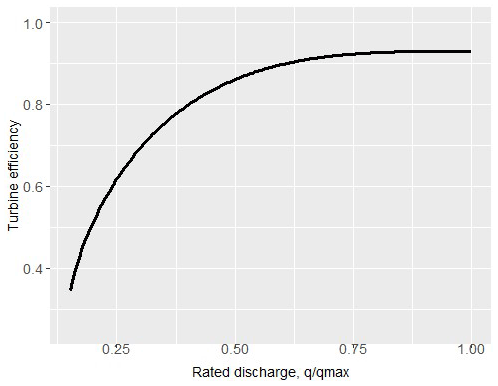
Figure 1 Efficiency curve for the Francis turbine applied in the hydropower system under study (analytically-derived relationship provided by Sakki et al., 2021, based on nomographs by Papantonis, 2008, p. 231).

3 Study area and data

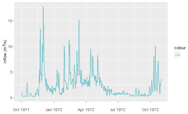
In the context of our analysis, we consider a run-of-river plant under study, in the upper course of river Achelous, Western Greece. The available hydrological information comprises spatially-averaged daily precipitation data from five representative meteorological stations, and daily streamflow data at the intake. The latter input is extracted by adjusting the observed inflows to a downstream site, i.e., Kremasta reservoir (Efstratiadis et al., 2014), by accounting for the ratio of the corresponding drainage areas (about 1:40). The common period of the two records extends over 39 years (May 1969 to December 2008). Figure 2 illustrates the adjusted flow time series, the mean annual value of which is 2.15 m³/s.

Figure 2 Streamflow time series at the intake for hydrological year 1971–1972.

Before proceeding with the forecasting problem, it is essential to specify the technical characteristics of the project. First, we estimate the environmental flow to be released downstream of the intake, in order to sustain the riverine ecosystems (Efstratiadis et al., 2014). Following the Greek legislation for SHPPs, this is defined as the 30 % of mean discharge of September, which here equals to 0.25 m³/s. The flow arriving at the intake is diverted through an open channel to a forebay and next conveyed to the power station through a penstock, thus creating an elevation difference of 150 m. In next computations, we consider this value as a constant net head, for simplicity, taking advantage of the quite large diameter of the penstock (1500 mm), causing minimal only hydraulic losses even at the maximum discharge capacity. We also apply a mixing of two Francis-type turbines, which characteristics are summarized in Table 1. The two capacities have been estimated through optimization, by maximizing the net annual profit of the system, estimated as the difference between the anticipated revenues from energy production and the depreciated costs of the electromechanical equipment (Sakki et al., 2021).

The operation policy of the SHPP is demonstrated in Fig. 3. This has been obtained by seeking for the optimal hierarchy of the two turbines, in order to maximize the power production across different discharge ranges. In particular, from 0.12 to 0.85 m³/s, i.e., the minimum flow of the small and large turbine, respectively, only the small turbine operates, while next, and up to the maximum discharge of the large turbine, i.e., 5.69 m³/s, it stops operating, since all diverted flow passes through the large turbine. For larger discharges up to the total system's discharge, the small turbine operates in its full capacity, which ensures a maximized overall efficiency. Under these assumptions, the project is expected to produce 47.5 MWh, on mean daily basis, thus ensuring a capacity factor of about 24 %.

Table 1 Design characteristics of the two Francis-type turbines.

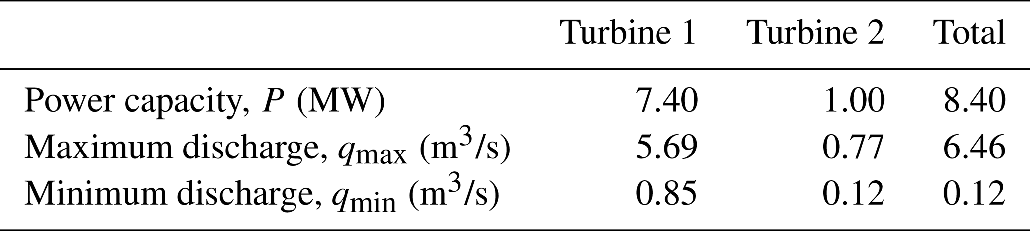
Figure 3 Optimal sharing of discharge conveyed to the two turbines and associated power production.

4 Application of alternative forecasting schemes

4.1 Generic framework

The consecutive conversions across SHPPs allows for establishing two alternative routes to the power forecasting problem, here employed on a day-ahead basis. The direct route aims at predicting the next-day energy production via regression models that use as explanatory variables past observations, in terms of power production and the past rainfall, as the sole source of hydrological data. On the other hand, the indirect route initially aims at predicting the day-ahead discharge, given that such data exist. The forecasted flows are next introduced to the operation model of the system, for extracting the forecasted energy. For each approach, we assess alternative forecasting schemes, in terms of model structure and data. In order to calibrate the free parameters of each model and evaluate their predictive capacity, we introduce a quite strict skill score in terms of the generic efficiency formula:

$$\begin{array}{}\text{(2)}& F=\mathrm{1}-{\displaystyle \frac{{\sum }_{t=\mathrm{1}}^n{\left(E_{t,\mathrm{obs}}-E_{t,\mathrm{forecast}}\right)}^{\mathrm{2}}}{{\sum }_{t=\mathrm{1}}^n{\left(E_{t,\mathrm{obs}}-E_{t,\mathrm{bencmark}}\right)}^{\mathrm{2}}}}\end{array}$$

where E_t,obs is the “observed” energy at day t, which is known from the simulation model, E_t,forecast is the forecasted value, which is estimated on the basis of past data $(x_{t-\mathrm{1}},x_{t-\mathrm{2}},\mathrm{\dots })$, and E_t,bencmark is a reference prediction, provided by a benchmark model. In the classical definition of efficiency, this coincides with the mean observation (thus the daily average energy production), yet here we also apply a stricter benchmark prediction, i.e., the so-called naïve forecasting model $E_t=E_{t-\mathrm{1}}$ (hereafter referred to as modified efficiency). The aforementioned expression ensures an efficiency up to 75.1 %, for the entire period of historical data (1969–2008; see Table 2). For each model, we also compute the marginal statistical characteristics of residuals, $w_t=E_{t,\mathrm{obs}}-E_{t,\mathrm{forecast}}$ (mean, standard deviation, coefficient of skewness) and the lag-1 autocorrelation, which is measure of dependence.

4.2 Direct (energy-based) approaches

In the direct approaches we use as independent variables (predictors) for the energy generated at time step (day) t+1, the past energy production, E, as well as the available hydrological data, by means of rainfall, p, from a representative meteorological station or the spatially-aggregated rainfall from a set of stations. After investigations, we concluded to a branched expression, that takes into consideration the appearance of a rainfall event at day t, which is expected to influence the generation of streamflow due to the increase of soil moisture over the basin:

$$\begin{array}{}\text{(3)}& E_{t+\mathrm{1}}=\left\{\begin{array}{ll}\mathrm{3.88}\left(E_t{)}^{\mathrm{0.54}}\right(E_{t-\mathrm{1}}{)}^{\mathrm{0.12}}(p_t{)}^{\mathrm{0.16}},& p_t>\mathrm{0.1}\mathrm{mm}\\ \mathrm{1.51}{\left(E_t\right)}^{\mathrm{0.63}}{\left(E_{t-\mathrm{1}}\right)}^{\mathrm{0.25}},& p_t\le \mathrm{0.1}\mathrm{mm}\end{array}\right.\end{array}$$

Following the typical split-sample approach, we estimated the seven model parameters by calibrating against the actual energy production values in the half of observations, and validating its predictive capacity in the other half. The skill scores in calibration and validation, expressed in terms of classical and modified efficiency, as well as the statistical characteristics of the model error are summarized in Table 2.

4.3 Indirect (flow-based) approaches

In the indirect approaches we aim to provide day-ahead forecasts of the discharge to feed the flow-energy conversion model, which is summarized in the diagram of Fig. 3. In this respect we use as predictors of streamflow at day t+1 the past streamflow and the rainfall. In order to account for the baseflow component of streamflow, we also extract the minimum value of last five days, q_min5, and the mean monthly value of the full data sample; these predictors were determined by following an input variable selection procedure (Galelli and Castelletti, 2013). We remark that the baseflow component may incorporate several slow-flow elements, associated with groundwater runoff, snow melting (which is quite significant, during the spring period) as well as the falling limb of floods. After investigations, we conclude to the parametric expression:

$$\begin{array}{}\text{(4)}& q_{t+\mathrm{1}}=\left\{\begin{array}{ll}{a}_{\mathrm{1}}\left(q_{\min \mathrm{5}}\right)+{\mathit{\beta }}_{\mathrm{1}}\left(q_t\right)+{\mathit{\gamma }}_{\mathrm{1}}\left(q_{\mathrm{mean}t}\right),& p_t<\mathrm{0.1}\mathrm{mm}\\ a_{\mathrm{2}}\left(q_{\min \mathrm{5}}\right)+{\mathit{\beta }}_{\mathrm{2}}\left(q_t\right)+{\mathit{\gamma }}_{\mathrm{2}}\left(q_{\mathrm{mean}t}\right)+\mathit{\delta }\left(p_t\right),& p_t\ge \mathrm{0.1}\mathrm{mm}\end{array}\right.\end{array}$$

As shown in Table 2, by employing a typical calibration on the basis of maximizing the efficiency of the simulated against the observed streamflows, in terms of day-ahead energy prediction we obtain a small only improvement with respect to the direct modelling approach, namely from 79.9 % to 80.7 % (for the full data). On the other hand, the model error characteristics are less satisfactory, since the forecasting model underestimates the energy production by about −3.8 MWh, on average, while with the direct approach the bias is negligible. This is due to the attempt of the calibration procedure to predict streamflows outside of the operational range of turbines, and particularly the peak flows, which result to large errors. Yet, these errors are beyond our concerns, since during these periods the system operates continuously in its nominal capacity.

In order to remedy the above shortcomings, we adjust the fitting metric, i.e., efficiency, to the turbine operation range (q_min, tot, q_max, tot), in order to ignore the errors that are produced from the flow forecasting model, if this correctly predicts that the flows being outside this range. Moreover, if the forecasted flow is inside the range, whereas the observed is outside, we only account from the distance from the two flow limits. Under this premise, the error is calculated as follows:

$$\begin{array}{}\text{(5)}& e=\left\{\begin{array}{l}{q}_{\max ,\mathrm{tot}}-q_{\mathrm{forecast}},q_{\mathrm{obs}}>q_{\max ,\mathrm{tot}}\text{ and }{q}_{\mathrm{forecast}}<q_{\max ,\mathrm{tot}}\\ q_{\mathrm{forecast}}-q_{\min ,\mathrm{tot}},q_{\mathrm{obs}}<q_{\min ,\mathrm{tot}}\text{ and }{q}_{\mathrm{forecast}}>q_{\min ,\mathrm{tot}}\\ q_{\mathrm{obs}}-q_{\mathrm{forecast}},q_{\mathrm{obs}}>q_{\min ,\mathrm{tot}}\text{ and }{q}_{\mathrm{obs}}<q_{\max ,\mathrm{tot}}\end{array}\right.\end{array}$$

The above error expression incorporates within calibration, apart from the hydrological data, the expert's knowledge about the technical properties of the system that affect the flow-energy conversions. The knowledge-based calibration approach, herein called Indirect Model B, ensures a clearly better skill score in terms of modified efficiency than the typical calibration approach (Indirect Model A), and good error properties as well (practically zero mean and autocorrelation).

An interesting question that arises is whether just a better day-ahead flow forecasting model that does not account for the operational characteristics of the system, would outperform the optimal model so far. In this respect, we apply a more complex approach from the Machine Learning (ML) family, namely a Deep Feedforward Neural Network (DNN). The DNN model is composed by three hidden layers with 128, 64 and 64 neurons, respectively, while the Rectified Linear Unit (ReLu) activation function is adopted for all neurons. As inputs, we use the streamflow of past 5 d and the rainfall of past two days. The model is fitted on the basis of Mean Square Error (MSE), for a number of 100 epochs, by using a batch size of 64.

In Fig. 4 we compare the actual and forecasted flow and energy values provided by the Indirect Model B and the ML approach, for hydrological year 1971–1972. Surprisingly, while the ML model ensures a much better fitting to the observed flows than the simple regression expression (4), (84 % vs. 63 %), the conversion to energy is rather disappointing. In particular, the classical efficiency metric is only 50.7 %, while the modified efficiency is strongly negative. Furthermore, the derived error properties are clearly non satisfactory (underestimation of the average energy up to 1 MW, quite large standard deviation, and, significant autocorrelation). The poor predictive capacity of the data-driven approach is attributed to the training procedure, in which we ignored the range of operation of the small hydroelectric plant, which is key feature of its management.

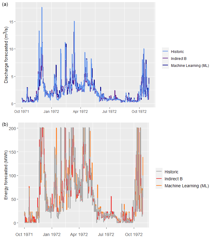
Figure 4 Comparison of historical vs. predicted time series obtained by two forecasting models (indirect B and ML) for (a) inflows and (b) energy production (hydrological year 1972–1973).

Table 2 Comparison of different forecasting schemes.

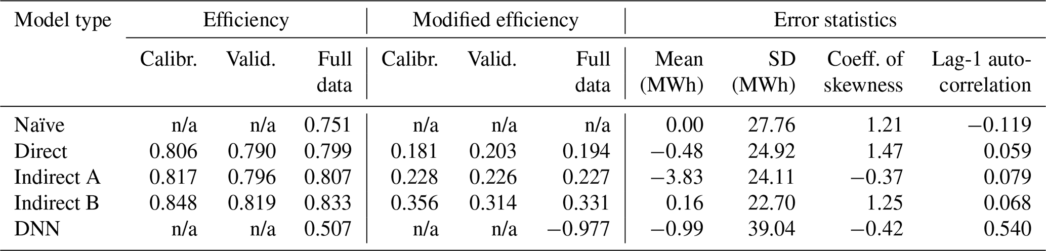
n/a: not applicable

5 Forecasting and uncertainty: reconciliation in practice

Predictive uncertainty is defined as the probability of occurrence of a predictand's value (in the particular case, energy production) conditional upon prior observations and knowledge, as well as on all the information we have obtained on that specific value from model forecasts (Coccia and Todini, 2011). A typical means to quantify the predictive uncertainty of a deterministic simulation model, is to add a random component (noise), w_t, to its output, y_t, where the random process w_t should be consistent with the statistical and stochastic regime of the associated residuals (Efstratiadis et al., 2015). In the generic case of autocorrelated errors, the process w_t can be obtained by a stochastic generator (e.g., Kossieris et al., 2019; Tsoukalas et al., 2018, 2020), or a statistical distribution model, provided that the errors do not exhibit significant dependencies in space and time. By generating a large enough set of random variables $y_{i,t}=y_t+w_{i,t}$, where $i=\mathrm{1},\mathrm{\dots },n$, we obtain an ensemble of n model realizations at each time step t, which allows for the detection of empirically-derived probabilistic quantities. This procedure is widely known as Monte Carlo simulation.

In our case, we use the more robust forecasting scheme (Indirect Model B) and provide n=100 realizations of the day-ahead energy at each time step (day), from which we get the median and the 10th and 90th largest values (quantiles) of forecasted energy production, as estimators of the 80 % empirical confidence intervals. Given that the observed residuals are uncorrelated, the errors are considered as a stationary process that follows a three-parameter gamma distribution (i.e., Pearson type III), which reproduces the mean value, μ_e the standard deviation, σ_e, and the coefficient of skewness, γ_e, of the entire sample of residuals (Table 2). We also implement the same analysis by applying seasonally-varying (cyclostationary) generation models, which account for the individual statistical characteristics per month (Tsoukalas et al., 2018). As shown in Table 3, these is a considerable difference of the statistical behavior of the error across different seasons, that is also reflected in the uncertainty of energy predictions. In Fig. 5 we compare the uncertainty bounds obtained from the two methods, for hydrological year 1971–1972. We observe that during the low-flow period, these bounds are substantially reduced, by accounting for the issue of seasonality. This indicates that the more detailed analysis, where the prediction error is represented as a cyclostationary process, is much more realistic.

In order to take advantage of the concept of uncertainty in practice, as would be made in a real-world energy market, we can determine alternative market policies in terms of quantiles. In particular, we can apply the upper, middle and low quantiles as representatives of a risky, mild and conservative forecast of the day-ahead energy, and evaluate them in economic terms, by assigning a unit profit value for delivering the energy produced up to the forecasted value, and a unit penalty for the deviations (i.e., deficits with respect to the forecasted value). For instance, we account for the 90 %, 50 % and 10 % quantiles and apply a fixed profit of EUR 60/MWh and a penalty value of EUR 50/MWh; the aforementioned values are representative of the recent system marginal price and price of deviations, respectively, of the Hellenic Electricity Market. Under this premise, the mild policy ensures a mean annual profit of EUR 0.86 million, the conservative EUR 0.81 million, and the risky EUR 0.43 million. This quick pseudo-financial analysis allows for comparing the different interpretations of a forecasting approach under uncertainty.

Table 3 Monthly statistical characteristics of residuals derived from the application of Indirect Model B.

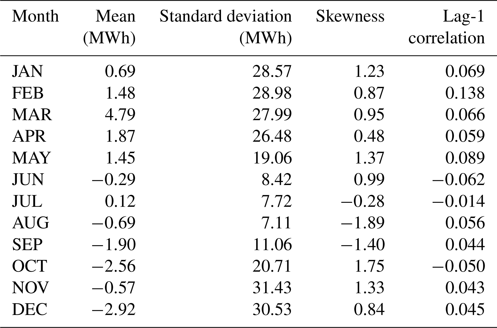
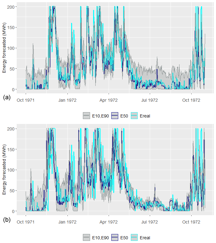
Figure 5 Comparison of actual energy production for hydrological year 1972–1973 with three characteristic prediction quantiles (10 %, 50 % and 90 %), by considering the error process as: (a) stationary and (b) cyclostationary.

6 Conclusions

This research aims to revisit the problem of day-ahead power forecasting in the case of small hydropower plants without storage capacity, which has received little attention so far. Taking as an example a typical project of this category, and by using simple yet effective modeling schemes, we attempt to revisit several issues that may have been well-addressed in the generic context of hydrological forecasting, but not in the specific case of SHPPs, namely: (a) the essential information as input to hydropower forecasting; (b) the advantages of the indirect forecasting approach, involving the use of a streamflow forecasting model, against the direct one, that does not account for the inflow input, but relies solely on the energy production data; (c) the importance of past precipitation data as exogenous predictor, providing macroscopic information about the catchment state (e.g. antecedent soil moisture conditions); (d) the training procedure and the skill score to be applied; and (e) the representation of the predictive uncertainty around the point forecast of day-ahead energy; (f) and the use of uncertainty-aware forecasts from the practicians' point-of-view (investors, power engineers, stakeholders).

Our investigations indicated that the proposed flow-based approach is more flexible and physically consistent, since it provides forecasts of the hydropower system's driver, i.e., the inflow arriving at the intake. We also revealed that apart from the inflow data per se, additional information should be introduced within prediction schemes in order to better reflect our hydrological knowledge, in terms of statistical characteristics. In the particular example, these were the mean monthly inflows and the past five-day average values, as representative of the long and short-term regime of the upstream catchment, respectively. However, it is worth mentioning that even a very good prediction of inflows (as quantified in terms of efficiency), does not guarantee an equally good performance in energy prediction (see Fig. 4). Equivalently important is the training procedure and the associated performance measure, where the system's characteristics, i.e., the range of operation of turbines, are embedded as inputs to calibration.

Key outcome of this research was also the quantification of uncertainty, by means of empirical quantiles, which were estimated through a Monte Carlo approach, after fitting a suitable probability distribution to the model residuals. This task, although proved to be simple and effective in its implementation, requires more careful examination, including analysis of the error properties and their seasonal variability, as well as could be benefited from more advanced concepts and tools, such as copulas and conditional non-Gaussian distributions (cf. Tsoukalas, 2018, for a development of this kind). Nevertheless, the interpretation of uncertainty is essential as a guidance for modelling energy market behaviors and providing decision support in the Target model era.