 | 09 Oct 2020
Development of an Electrical Resistivity Tomography Monitoring Concept for the Svelvik CO2 Field Lab, Norway
Wolfgang Weinzierl
Bernd Wiese
Dennis Rippe
Cornelia Schmidt-Hattenberger
Within the ERA-NET co-funded ACT project Pre-ACT (Pressure control and conformance management for safe and efficient CO2 storage – Accelerating CCS Technologies), a monitoring concept was established to distinguish between CO2 induced saturation and pore pressure effects. As part of this monitoring concept, geoelectrical cross-hole surveys have been designed and conducted at the Svelvik CO2 Field Lab, located on the Svelvik ridge at the outlet of the Drammensfjord in Norway. The Svelvik CO2 Field Lab has been established in summer 2019, and comprises four newly drilled, 100 m deep monitoring wells, surrounding an existing well used for water and CO2 injection. Each monitoring well was equipped with modern sensing systems including five types of fiber-optic cables, conventional- and capillary pressure monitoring systems, as well as electrode arrays for Electrical Resistivity Tomography (ERT) surveys.
With a total of 64 electrodes (16 each per monitoring well), a large number of measurement configurations for the ERT imaging is possible, requiring the performance of the tomography to be investigated beforehand by numerical studies. We combine the free and open-source geophysical modeling library pyGIMLi with Eclipse reservoir modeling to simulate the expected behavior of all cross-well electrode configurations during the CO2 injection experiment. Simulated CO2 saturations are converted to changes in electrical resistivity using Archie's Law.
Using a finely meshed resistivity model, we simulate the response of all possible measurement configurations, where always two electrodes are located in two corresponding wells. We select suitable sets of configurations based on different criteria, i.e. the ratio between the measured change in apparent resistivity in relation to the geometric factor and the maximum sensitivity in the target area. The individually selected measurement configurations are tested by inverting the synthetic ERT data on a second coarser mesh. The pre-experimental, numerical results show adequate resolution of the CO2 plume.
Since less CO2 was injected during the field experiment than originally modeled, we perform post-experimental tests of the selected configurations for their potential to image the CO2 plume using revised reservoir models and injection volumes. These tests show that detecting the small amount of injected CO2 will likely not be feasible.
- Article
(4269 KB) - Full-text XML
- BibTeX
- EndNote


Carbon Capture and Storage is considered an important technology to contribute to a carbon neutral society and is again receiving increased attention in the efforts to reduce CO2 emissions (Bui et al., 2018). To ensure safe operation of such CO2 storage projects, reliable monitoring technologies are required (Jenkins, 2020). Electrical resistivity tomography (ERT) is a long established geophysical technique to image the resistivity distribution in the subsurface which is subject to potential process induced resistivity changes. Due to the generally high electrical resistivity contrast between CO2 and formation water, ERT can be considered as one of the most effective geophysical techniques for the long-term monitoring of CO2 distribution and migration in subsurface storage reservoirs (Yang et al., 2014; Schmidt-Hattenberger et al., 2016).
To further develop CO2 storage monitoring procedures, a field experiment was planned at the Svelvik CO2 Field Lab, a small scale test site located on the Svelvik ridge in Norway (Ringstad et al., 2019). A main goal of the experiment was to discriminate pressure- and saturation induced effects, particularly on seismic measurements. In the first stage of the experiment, brine was injected to calibrate a rock physics model used to determine the pressure influence on seismic velocities. In a second stage, CO2 was injected. From the difference of both stages reservoir pressure and saturation should be determined. ERT was intended to act as complementary measurement in the second stage of the experiment, to provide an independent estimation of CO2 plume shape and saturation.
ERT measurement configurations consist of four electrodes, of which two are used for current injection (labeled A and B) and two are used to measure the resulting potential (labeled M and N). A key problem of the application of ERT in the subsurface is the selection of a suitable set of measurement configurations for the given problem. A total of 64 electrodes was installed in 4 newly drilled wells surrounding an existing well used for brine and CO2 injection. For a number of n(64) subsurface electrodes, there exists (≈ 1.9 million) independent configurations when reciprocal configurations are excluded (Noel and Xu, 1991). Each configuration has unique features, as e.g. the associated geometric factor, and a specific sensitivity for different parts of the subsurface model. The aim of this study is to reduce the required number of measurements by selecting the most sensitive electrode combinations to limit the required run time for a schedule.
The injection of CO2 is a dynamic process. After injection start rapid changes of saturation occur, while the plume tends to stabilize with longer injection time. A trade off has to be made between information due to a limited number of observations and the observation of a dynamic process, with each single observation showing a different state due to the ongoing plume migration.
As shown by Bing and Greenhalgh (2000), configurations where current and potential electrodes are distributed between a pair of wells, i.e. AM–BN configurations produce the highest image quality. AB–MN are generally considered inferior because the geometric factor turns from positive to negative in a discontinuous way, leading to low potential readings. They have however a potentially beneficial sensitivity distribution in the imaging of laterally elongated resistivity anomalies (Zhou, 2019) as would be expected e.g. for CO2 trapped beneath a cap rock.
Different approaches to select suitable measurement configurations have been proposed and used. Stummer et al. (2004) were the first to introduce experimental design for ERT measurements and to present a strategy for optimizing the measurement schedules for surface measurements. The method was expanded to homogeneous subsurface problems for cross-well geometries by Coscia et al. (2008). In this context, Wagner et al. (2015) incorporated the position of electrodes itself in the optimization scheme. Alternative approaches focus on finding an optimal model resolution for a particular area of the problem space (Wilkinson et al., 2006; Loke et al., 2014). Uhlemann et al. (2018) expanded on their work by integrating the optimization of measurement configurations and electrode configurations into a combined approach, which could be useful for future sites where the electrodes are not yet installed. A common advantage of these optimization strategies is the consideration of linear independence of sensitivities, either directly or by maximizing the diagonal elements of the resolution matrix. However, this comes at the cost of computational intensity and memory requirements, i.e. multiplication of large matrices and solving of large, dense equation systems are required. Other strategies rely on optimizing the sensitivity of a measurement schedules by directly utilizing the Jacobian matrix of the problem (Hennig et al., 2008; Athanasiou et al., 2009) and considering an estimate of the data error in the optimization problem (Wilkinson et al., 2012).
The work presented here follows a similar approach by optimizing the measurement configurations based on their sensitivity and associated geometric factor, but also considers the performance over the course of an injection experiment. Whereas our optimization focuses on the end state of the CO2 injection, it could be extended to intermediate time steps to determine optimized measurement configurations to best image the dynamics of the injection process.
For CO2 storage projects, generally a high amount of information should be available in the form of numerical reservoir models, incorporating petrophysical information from well logs and structural information from site exploration. Therefore, in this study, known geological data is incorporated into a reservoir model to describe the CO2 migration in the sub-surface. The modeled CO2 saturations are converted into an increase in bulk resistivity according to Archie's Law (Archie, 1942).
Prior to the CO2 injection, a potential injection regime was simulated with a site adapted reservoir model. The resulting plume was transferred to an electrical resistivity increase. The increase was observed by three ensembles comprising different electrode configurations. The specific characteristics of the inversion results were assessed.
After the experiment had taken place, the reservoir model was updated with information acquired during the installation and results obtained from the injection experiments. The measured schedules were tested using the revised model including site-specific information on the dynamic behavior.
The Svelvik CO2 Field Lab is located on the Svelvik ridge peninsula, approximately 50 km SW of Oslo, Norway (Fig. 1a). The ridge is classified as a glaciofluvial-glaciomarine terminal deposit. The site is characterized by highly variable grain size distribution with pebble and cobble beds in the overburden. At the site, but outside the area addressed in this paper, in 2011, 1.7 t of CO2 were injected in to a shallow aquifer at 30 m depth (Barrio et al., 2014).

Figure 1(a) Location of the Svelvik CO2 Field Lab on the Svelvik ridge. (b) Detailed view of the test site with locations of the monitoring wells (M1–M4) and the injection well Svelvik #2.
In July 2019, the Svelvik CO2 Field Lab was extended by drilling four 100 m deep monitoring wells (M1–M4) around the existing well Svelvik #2. This legacy well was later used for injection during the planned water and CO2 injection experiments (Fig. 1b). The monitoring wells were equipped with state of the art sensing systems, including five types of fibre-optic cables, conventional pressure sensors at reservoir level, fluid- and gas sampling capillaries, as well as a capillary pressure monitoring system (Wiese et al., 2020). As schematically illustrated in Fig. 2, an array of 16 electrodes with equidistant spacing of 5 m, was installed in each well, from 23 down to 98 m depth (below ground level).
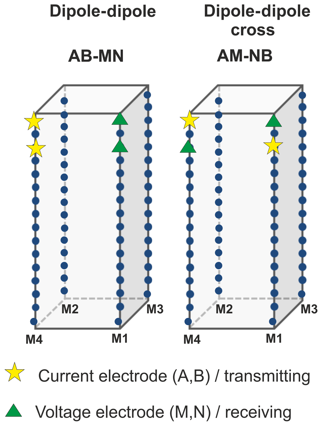
Figure 2Schematic diagram (not to scale) of the ERT array installed at the Svelvik CO2 Field Lab. Shown as well are typical electrode configurations used in cross-well imaging.
3.1 ERT Theory and Modeling
ERT data is typically acquired in four point configurations, i.e. the electric current I is injected between two electrodes generally referred to as A and B. The electric potential U is measured between a second pair of electrodes often referred to as M and N. The apparent electrical resistivity is then given as
where k is the geometric factor that takes into account the distance and arrangement of current and potential electrodes (Telford et al., 1990). Large geometric factors correspond to low potential readings with unfavorable signal-to-noise ratio and therefore, in general, higher relative measurement errors.
Most commonly, collected ERT data are inverted to determine the subsurface model which minimizes the discrepancy between observed and modeled data (Günther et al., 2006). An important component in the inversion problem is the Jacobi Matrix, which contains partial derivatives of the model responses for all individual configurations fi with respect to the model parameters mj (McGillivaray and Oldenburg, 1990). The Jacobian matrix Jij is therefore given as
and represents the influence of a particular model cell of the numerical domain on the simulated apparent resistivity.
An empirical relationship describing the electrical resistivity of fluid-filled rocks was discovered by Archie (1942) in the form of
where Rrock is the bulk electrical resistivity, Φ is the porosity, Sw is the water saturation, and Rw is the brine resistivity. The factor a is the tortuosity factor, m is the cementation exponent, and n the saturation exponent.
Often referred to as Archie's second law, the resistivity index RI i.e the ratio between electrical resistivity of the partly saturated rock R and the brine saturated rock R0 can be calculated as
where and Sw is the water saturation. It can be related to the CO2 saturation , which is not part of the original formulation of Archie's law. Using RI instead of the absolute resistivity is only possible when baseline data is available. It has the advantage that the natural variability in the subsurface is leveled out and does not need to be resolved.
3.2 Modeling Concept
3.2.1 Geological model
The structural reservoir model is based on the interpretation of two intersecting 2D seismic profiles acquired during a previous appraisal and injection campaign on the test site in 2010 (Bakk et al., 2012; Grimstad et al., 2018). Using the main structural horizons and interpretation of the logging campaign the aquifer and cap-rock zones were distinguished. The structure consists of equally thick layers with a small dip of 2.7 %. At 65 m depth an aquifer has been identified as target formation from analyzing grain size distributions and gamma ray logs. Above 65 m the borehole logs show a slightly reduced porosity and permeability which is interpreted as a barrier for CO2.
The main petrophysical properties determining the subsurface migration of the injected CO2 are porosity and permeability. We determine these parameters in an approach also detailed by Wuestefeld and Weinzierl (2020), using the Greenberg-Castagna relation (Greenberg and Castagna, 1992) given as
Parameters ac=5.81, , and are chosen according to the highly unconsolidated environment, similar to the geologically young Gulf Coast reservoirs like the Frio formation. VCL is the clay content, and the required P-wave velocity VP was taken from sonic log from the previous appraisal campaign. The resulting porosity is on average 26 %.
Permeabilities κ are derived from the porosities using the Kozeny-Carman equation (Carman, 1997) given as
with mineral sphere diameters d=6 mm obtained from the coarse- to fine grain-size distributions. The tortuosity (τ≈0.25)-dependent factor B=0.23 has been calibrated by a previous hydraulic conductivity test in between 64 and 66 m depth, which determined a permeability of roughly 150 mD. Permeabilities are then calculated over the complete model depth using the estimated porosities. While a rigorous derivation of permeabilities would include a grain size as well as a clay content dependent definition, we keep the parameters used constant over the entire static model.
The determined geophysical parameters have been incorporated in a 3D geological model generated with Petrel. The one-dimensional properties are propagated throughout each individual stratum of the model. Additionally, we have populated the strata of the geological model with resistivity values from a well log acquired during the previous appraisal campaign.
The horizontal cell size is 5 m. The vertical cell size varies between 1 m in the reservoir region (51–71 m depth) and up to 18 m above the glacial till layer. The horizontal extent is 195 m × 195 m, the depth between 0 and 90 m. The increased content of fine material above 65 m increases the capillary entry pressure, which is set to 5 bar. It therefore represents an effective barrier for CO2 in the model. Following well construction data the injection interval is 1 m, which is shifted by a few cm to screened model depths between 65.5 and 66.5 m.
3.2.2 Pre-Experiment Eclipse Simulation
The reservoir simulation is set up with Eclipse 300 (Schlumberger, 2015). The CO2 injection was modeled for an injection rate of 200 Sm3 d−1, resulting in a cumulative mass of 23 t of CO2 after 57 d of injection. This is consistent with an initial feasibility study of geophysical monitoring at the Svelvik CO2 Field Lab, which had been used for synthetic controlled source electro-magnetics (CSEM) and full waveform inversion (FWI) studies (Eliasson et al., 2014), thus allowing future comparison of the different geophysical methods. Additional reservoir modeling as part of the feasibility study used a lower injection rate of 50 Sm3 d−1 due to the risk of seal fracture at higher injection rates. Subsequent studies, however, suggested that a maximum injection rate of up to 300 Sm3 d−1 over a period of 28 d is possible without exceeding the bottom-hole pressure (BHP) limit of 10 bar in the injection well (Grimstad et al., 2018).
Figure 3a shows the resulting CO2 saturation after injection of 23 t of CO2 along a NS cross-section at x=92.5 m, which is at the location of the injection well. The largest part of the gaseous CO2 is contained below the sealing stratum. Some leakage into the overburden is observed. The CO2 remains contained however. The initial simulation performed prior to the experiment is discarding solubility effects of CO2 in the formation water.
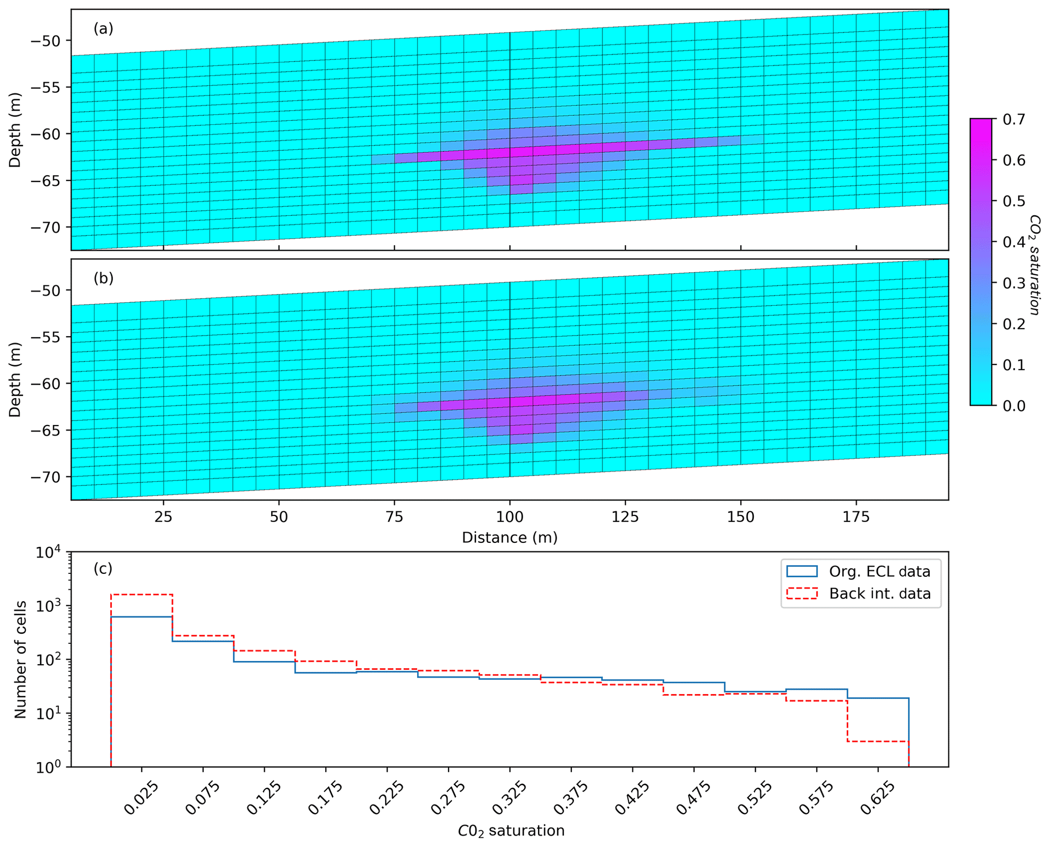
Figure 3(a, b) Slice through 3D Eclipse reservoir model after the injection of 23 t of CO2. (a) Original CO2 saturation data. (b) CO2 saturation data after interpolating onto the unstructured grid, and then back-interpolating onto the structured Eclipse grid. (c) Histogram showing the CO2 distribution for original and back-interpolated saturation data. The bin width is 5 %.
3.2.3 ERT Forward Modeling Workflow
To perform the ERT modeling we use the free and open-source library pyGIMLi (Rücker et al., 2017). pyGIMLi is able to utilize unstructured grids, based on tetrahedral elements. We generate a suitable unstructured grid using the software Gmsh (Geuzaine and Remacle, 2009). This allows for finer meshing and subsequently more accurate ERT forward simulations.
The mesh consists of two regions: one finely meshed, inner region that acts as inversion region, that has the same x and y extent as the Eclipse grid. The z extent is from 10 to 110 m depth. The larger outer region is necessary so that source positions of the electric field (current electrodes) can assumed to be constant when considering the boundary conditions (Rücker et al., 2006). It is meshed more coarsely and symmetrically located around the inner region. The x and y extent of the outer region is 1000 m. It extends from 0 to 300 m depth.
We use the cell center coordinates for 3D linear interpolation of relevant parameters (porosity, CO2 saturation, electrical resistivity) from the structured Eclipse grid to the unstructured pyGIMLi mesh. To quantify the error the interpolation between the grids introduces, we again back-interpolate on the structured grid (Fig. 3b). Some interpolation errors are observed. Especially the thin, high saturation layer in 65 m depth is eroded.
A saturation histogram with a bin width of 5 % is shown in Fig. 3c. Due to interpolation errors, the CO2 migrates from higher to lower concentrations, therefore higher concentrations are decreased, and more cells of lower concentration appear. Additionally, we have calculated the contained CO2 volume in both grids neglecting potential pressure differences i.e. calculating the sum of cell volume times CO2 cell saturation for all model cells. The difference between both grids is ≈0.3 %, for the injection of 23 t of CO2.
Figure 4 shows the structured Eclipse grid populated with electrical resistivity values. Together with the CO2 saturations, as illustrated in Fig. 3 we construct electrical resistivity models for the ERT forward modeling problem using Eq. (4), for all reservoir simulation time steps. The saturation exponent n is assumed to have a value of 2, which generally represents a good estimate for oil-free sediments (Mavko et al., 2009).

Figure 4Reservoir model grid populated with electrical resistivity values and locations of the monitoring and injection wells. The injection well is located at x, y=92.5 m. The green wire frame represents the outer surface of the unstructured inversion region. Shown as well, is a slice through the 3D reservoir model between well M2 and M1 in terms of the resistivity index R∕R0 after the injection of 23 t of CO2.
Shown as well in Fig. 4 is a slice through the NW–SE trending diagonal between observation wells M2 and M1. The slice shows the resistivity index after the simulated injection of 23 t of CO2. In the following, models and results will be presented as a slice along this axis. Distance refers to distance along the diagonal.
3.2.4 ERT Measurement Schedule Selection
For the ERT schedule selection we have used the last simulation time step. As suggested by Bing and Greenhalgh (2000), we simulate all configurations where always a pair of current and potential electrodes is located in two corresponding wells i.e. AM–BN configurations. Additionally, we have included configurations where both current and potential electrodes are located in two corresponding wells i.e. AB–MN configurations. Crossed dipoles and reciprocal measurements have been excluded. We also excluded configurations where the geometric factor is larger than 10 000. This leads to 84 280 potential measurement configurations.
To select appropriate configurations, we have developed and tested two ranking criteria to image the CO2 distribution. A volume of interest (VOI) around the simulated CO2 plume is defined. The VOI has a spatial extent of 75 to 105 m in the x- and y direction. In the z direction the VOI has a range from 55 to 75 m depth. The injection well is located at m.
Schedule 1 (geometry optimized schedule) aims to minimize the influence of the geometric factor and maximize the measured voltage difference in response to the injected CO2. The electrical resistance R is calculated for the pre-injection state and after the injection of 23 t of CO2. The difference is divided by the geometric factor. Individual configurations i are therefore ranked according to
These schedules can also be split into groups of AM–BN and AB–MN configurations respectively.
Schedule 2 (sensitivity optimized schedule) is selected by calculating the sensitivity for each individual electrode configuration. Similar to Hennig et al. (2008), the aim is to maximize the sensitivity in a section of the model space. Defining a weighting vector wj which is one, when the cell center of the model cell lies within the VOI and zero otherwise. Individual configurations i are then ranked according to
where Ji: is the sensitivity of an individual electrode configuration for all model cells, extracted as a vector from the Jacobian matrix. Vj is the volume of the jth model cell, m is the number of model cells.
The volume is already included implicitly in the calculation of the sensitivity (Geselowitz, 1971). The mesh is locally refined around the electrodes, so the cells grow away from the electrodes. By multiplying with the cell volume additional weight is given to cells further away from the electrodes.
Schedule 3 (comparison/random schedule) is comprised as a comparison to the proposed selection criteria. From all possible cross-well AB–MN and AM–BN configurations it is pseudo-randomly chosen by selecting every ith generated configuration so that the selected number reaches the desired comparison size. This creates a wide range of configurations with different electrode spacings and geometric factors.
4.1 Pre-Experimet Optimization
To test the proposed criteria, we have selected 1000 members using the ranking methods. For the pseudo-random selection we have likewise generated 1000 configurations i.e. taking every 161th configuration. The schedules are tested using electrical resistivity models as exemplarily shown in Fig. 4. The response of the schedules is determined by solving the ERT forward problem for each time step. The obtained numerical data are then inverted on a coarser mesh. Since we are interested in imaging the CO2 induced changes, results are presented in terms of the resistivity index. Since we are interested in the relative performance of the measurement schedules, we consider noise free data. The Chi2 data misfits for the CO2 containing inversion result are given in the respective figure captions.
The geometry optimized schedule (Fig. 5a) resolves the spatial extent of the resistivity increase outside the observation wells. However, the maximum RI is approximately 1.75 and thus underestimating the resistivity increase observed in the original model. The sensitivity optimized schedule (Fig. 5b) resolves the plume between the observation wells, but hardly outside. The recovered RI is approximately 4, close to the original model. Some numerical artifacts are produced, especially around the electrodes, but also close to the top of the inversion region. The overview schedule (Fig. 5c) shows increased resistivity in the relevant area, but the footprint of the CO2 is unrealistically small. Also the shape of the plume is resolved less well compared to the previously discussed schedules. The peak recovered RI is approximately 3 and therefore closer to the synthetic reality than the geometry optimized schedule. A inversion artifact is produced at the top of the model between the two observation wells, which is outside the area of coverage however.
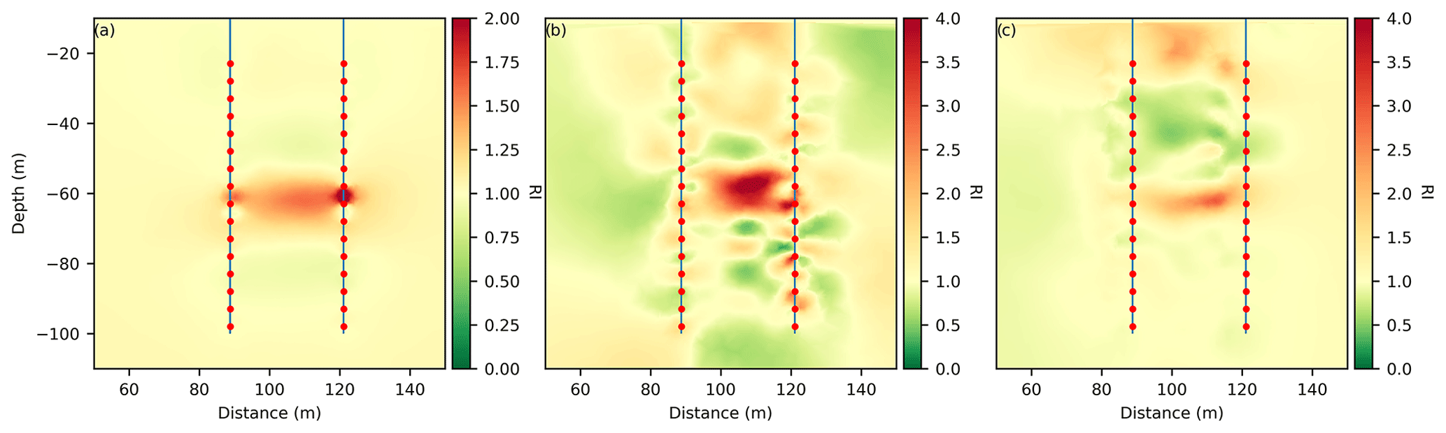
Figure 5Inversion results for selection criteria. 1000 Configurations have been selected for each configuration ensemble. (a) Geometry optimized schedule. (b) Sensitivity optimized schedule. (c) Overview/random schedule. Note the adjusted color scale for (a). The Chi2 misfits for the inverion result containning the CO2 plume are (a) 0.11, (b) 0.54, (c) 0.32.
4.2 Field Injection Experiment
The CO2 injection experiment took place between 24 October and 5 November 2019. Approximately 1.7 t of CO2 were injected instead of the originally modeled 23 t. Figure 6a shows the CO2 injection rate during the field experiment. CO2 injection was carried out with an injection rate of approximately 10 kg h−1 and has been paused during the weekend. For the injection experiment we have selected 2500 AM–BN as well as 2500 AB–MN configurations using the geometry optimized criterion discussed in the previous section. Due to an error, only 1992 configurations have been selected for the sensitivity optimized schedule.
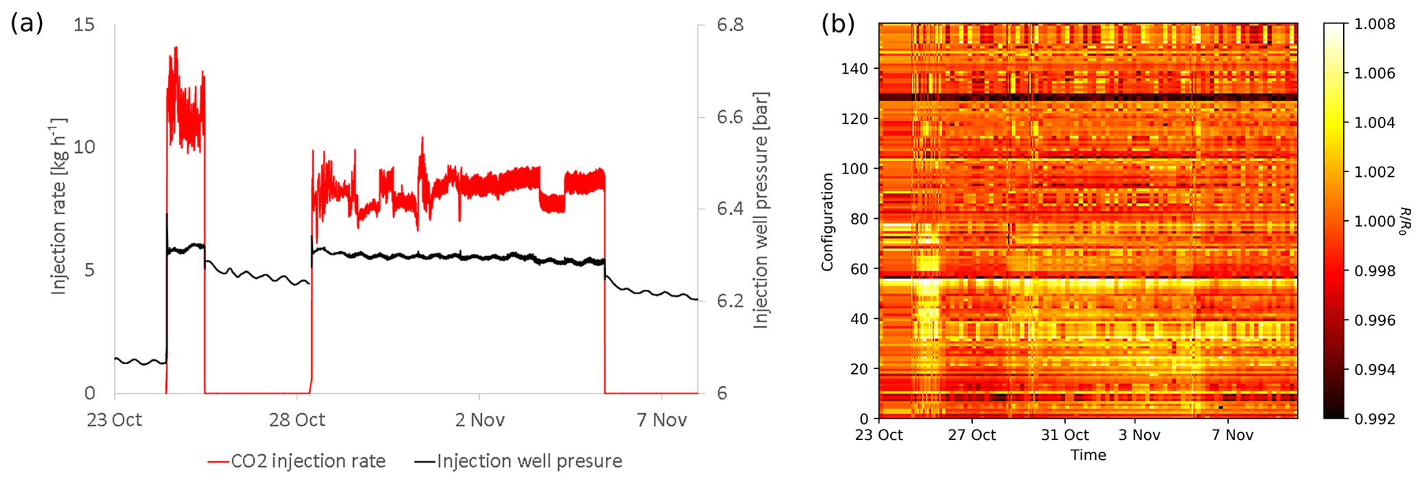
Figure 6CO2 injection rate during the field experiment. Approximately 1.7 t of CO2 have been injected. (b) Ratio of measured apparent resistivity between baseline- and subsequent measurements during the CO2 injection. Shown are 168 geometry optimized AB–MN configurations measured on the between wells M3 and M4 (NS axis).
So far, given the small amount of injected gas compared to the modeled scenario, we have not been able to image the potential CO2 plume inverting the collected ERT field data. Weak indications of CO2 induced effects are apparent in the time series of individual configurations (Fig. 6b). The increases are generally smaller than 1 %. The increases in apparent electrical resistivity mostly subside over the weekend, so that the experiment could be considered as two separate injection campaigns.
Applying the above mentioned reservoir model to an injection of 1.7 t shows that detection should still have been possible using the measured schedules. Results are shown in Fig. 7 for (a) the geometry optimized schedule AM–BN, for (b) the geometry-optimized schedule AB–MN, and (c) for the sensitivity optimized schedule. Both geometry optimized schedules resolve an RI value of approximately 1.1. The AB–MN configurations better resolve the elongated plume shape, but also produce erroneous resistivity increases surrounding the actual CO2 anomaly. The sensitivity optimized schedule resolves an RI value of 1.3.
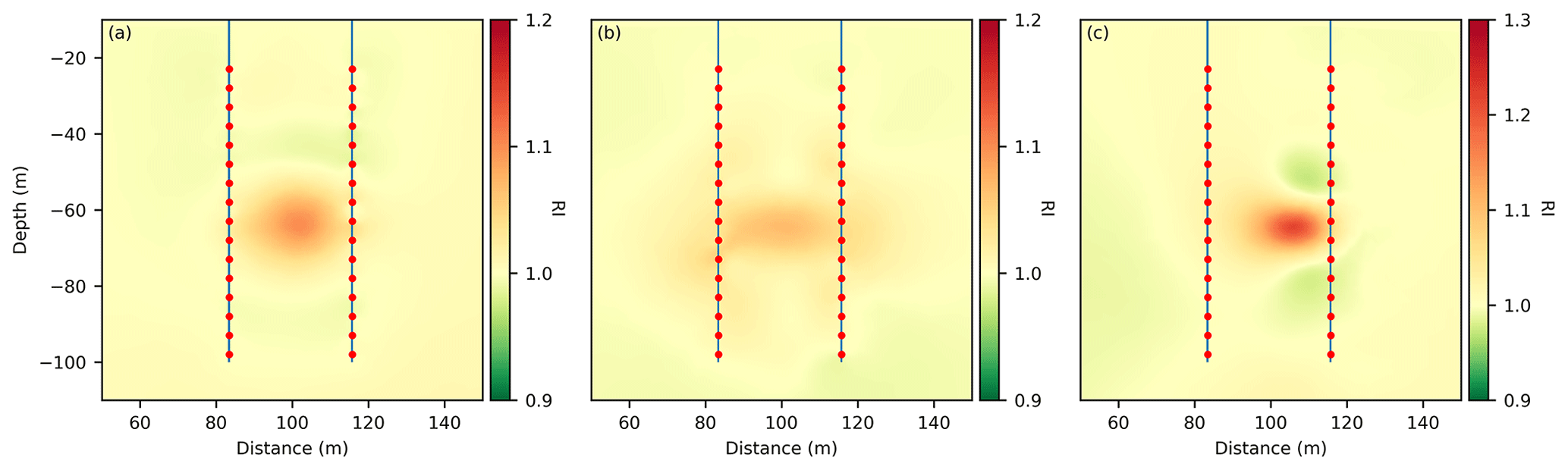
Figure 7Inversion results using the field schedules on the pre-experiment model for 1.7 t of CO2 injection. (a) Geometry-optimized AM–BN schedule. (b) Geometry optimized AB–MN schedule. (c) Sensitivity optimized schedule. Note the adjusted color scale for (c). The Chi2 misfits for the inverion result containning the CO2 plume are (a) 0.041, (b) 0.023, (c) 0.315.
Field observations and subsequent inversions showed only resistivity changes in the sub-percent range. This leads us to revise the reservoir model as will be outlined below.
4.3 Post-Experiment Evaluation
The horizontal reservoir permeability has been re-calibrated, such that the pressure increase during the water injection is about 0.5 bar and during CO2 injection is about 0.3 bar, which corresponds to the observed values during the brine injection experiment. The calibrated permeability in the storage horizon is around 1200 mD, which is eight times higher than initially estimated using the Kozeny-Carman equation. The horizontal and lateral grid size has been refined to 2.5 m, for more accurate reservoir simulations. The vertical grid size is maintained at 1 m. Additionally, the solubility of CO2 in the formation water is considered in the Eclipse reservoir simulation.
The revised reservoir simulation aims to reproduce the field injection as closely as possible. CO2 is injected with the real injection rate and paused at the weekend. In the simulation the CO2 completely dissolves during the injection free days. Figure 8a shows the end state of the CO2 injection. The CO2 plume has a lateral extent of 10 m and a thickness of 1 m. The maximum CO2 saturation is approximately 0.4.
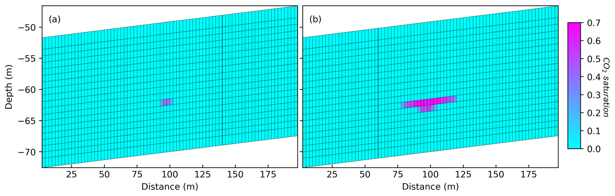
Figure 8(a, b) Slice trough the 3D Eclipse grid at x=92.5 m, showing the simulated CO2 cell saturation for (a) 1.7 t and (b) 23 t injected CO2 respectively.

Figure 9Slice through the 3D reservoir model in terms of resistivity index R∕R0 for 1.7 t of CO2 injection. (a) CaCO3 bearing aquifer. (b) CaCO3 free aquifer.

Figure 10Inversion results in terms of the resistivity index R∕R0 for 1.7 t of CO2 injection. (a, b) Geometry optimized schedule AM–BN, (c, d) geometry optimized schedule AB–MN, (e, f) sensitivity optimized schedule. (a, c, e) CaCO3 containing aquifer. (b, d, f) CaCO3 free aquifer. The Chi2 misfits for the inverion result containning the CO2 plume are (a) 0.135, (b) 0.137, (c) 0.007, (d) 0.005, (e) 0.032, (f) 0.031.
For comparison, Fig. 8b shows the hypothetical case, if the originally modeled 23 t of CO2 would have been injected in a longer field experiment. The lateral extent is comparable to the original simulation shown in Fig. 3. The thickness is about one fifth of the original estimate.
To estimate the effect of dissolved CO2 on the bulk electrical resistivity we use the full Archie equation (Eq. 3). Saturation exponent n and cementation exponent m are set to have a value of 2, which is typically assumed in applications of the Archie equation for silicate rocks Mavko et al. (2009). A lower cementation factor might have also been justified for the unconsolidated sediments at the Svelvik test site. The saturation exponent also can be lower in shale containing sands, but the effect is diminished for saline waters which can be found at the test site. In this sense the assumed parameters represent an optimistic scenario for the magnitude of the CO2 induced resistivity change.
The amount of dissolved CO2 is calculated by Eclipse in kg kg for each model cell. The brine electrical conductivity is calculated with PHREEQC and the Pitzer database. Fjord water is simulated as 0.5 % NaCl solution with a pH value of 7.2 at 8 ∘C. CO2 free Fjord water has an electrical conductivity of 6 mS cm−1 at temperature of 8 ∘C. We calculate the fluid conductivity for concentrations of CO2 in discrete steps corresponding to 0.0, 0.1, 0.2, 1, 3, 5, 7, and 9 bar partial pressure of CO2. We consider two possible cases:
Case 1 considers the presence of CaCO3 as a solid phase in the PHREEQC model, which is likely considering the glaciofluvial-glaciomarine setting. CO2 injection causes the dissolution of calcite, if present. For equilibrium of the formation water with calcite the additional calcium and carbonate ions cause a higher conductivity compared to calcite free conditions. In this case the brine conductivity increases considerably from the base value of 6 to 8.7 mS cm−1 for 9 bar partial CO2 pressure. The solubility for CO2 also increases, but only slightly by 5 %.
Case 2 assumes no CaCO3 in the formation. In this case the brine conductivity increases only due to increased carbonic acid from 6 to 6.1 mS cm−1.
Figure 9 shows the resulting RI values for 1.7 t of CO2 injection. Figure 9a shows the case for an CaCO3 bearing aquifer (case 1). A zone of reduced resistivity with RI values of approximately 0.75 is observed around an area of increased resistivity with RI values of approximately 1.4. Figure 9b shows the case of a CaCO3 free aquifer (case 2). No significantly reduced resistivity values can be observed. Peak RI values are approximately 1.9.
Using the revised reservoir models, numerical data is again generated for the simulated injection of 1.7 t of CO2 for the schedules measured during the field experiment. Figure 10 shows the respective inversion results. Panels in the left column show the case of a CaCO3 bearing aquifer. Panels in the right column show the results for a CaCO3 free aquifer. Panels show (a, b) geometry optimized AM–BN, (c, d) geometry optimized AB–MN, and (e, f) sensitivity optimized configurations respectively. For the case of a CaCO3 bearing aquifer all three schedules show an effective reduction in apparent resistivity values. For the geometry-optimized AB–MN configurations the reduction is smaller compared to the other two schedules. The inversion is not able to distinguish between the outer zone of resistivity reduction and the increase in the center of the anomaly. For the case of a CaCO3 bearing aquifer, all three schedules resolve resistivity increases of approximately 1.03. Again the AB–MN configurations show the lowest resolved amplitude.
5.1 Coupled Reservoir- and ERT modeling workflow
We have developed a coupled modeling workflow including reservoir simulation, petrophysical translation to electrical properties and geoelectrical forward simulation. This is followed by conventional smoothness-constrained inversion of the process-based synthetic ERT data sets. The conversion from a structured to an unstructured grid introduces some interpolation errors, but generally the CO2 distributions are accurately represented.
5.2 Performance of Selection criteria
The numerical results show that the coupled reservoir and ERT modeling can improve the understanding of ERT measurement schedule performance in the context of CO2 storage. The presented selection criteria show better imaging performance compared to a pseudo-random overview selection of configurations, using only a limited number of measurement configurations. The sensitivity optimized schedule produces the closest reproduction of the CO2 induced resistivity increase. The geometry optimized schedule is best able to resolve the spatial extent of the resistivity anomaly, but resolves lower peak RI value than both other investigated schedules.
5.3 ERT Imaging at the Svelvik CO2 Field Lab
We have investigated the performance of the selected schedules at the Svelvik CO2 Field Lab, using reservoir models refined after the experiment. The schedules struggle to resolve the more complex resistivity behavior introduced by the revised reservoir models. For the case of 1.7 t of injected CO2 the schedules only resolve minor amounts of increased resistivity. The smaller thickness of the simulated CO2 plumes likely plays an important role in the difficulty to resolve the resistivity anomalies. The potential presence of carbonates further lowers the predicted magnitude of CO2 induced resistivity anomalies, hindering detection. Given the small changes resolvable using numerical data, detection of the small amount of injected CO2 detection using the field data will likely prove infeasible.
Although the ERT imaging at the Svelvik CO2 Field Lab so far has not been able to resolve trapped CO2 in the target aquifer, we have gained better understanding of the test site through revised reservoir modeling.
The study shows that monitoring small scale CO2 injections using ERT has challenges associated with it. Accurate reservoir models can help to better plan such experiments in the future.
The data that support the findings of this study are available from the corresponding author, upon reasonable request.
TR compiled the manuscript and implemented the ERT simulation and inversion. WW constructed the original reservoir model including the petrophysical permeability estimation. BW refined the reservoir model and performed the PHREEQC calculations. DR and CSH advised and proof read the manuscript.
The authors declare that they have no conflict of interest.
This article is part of the special issue “European Geosciences Union General Assembly 2020, EGU Division Energy, Resources & Environment (ERE)”. It is a result of the EGU General Assembly 2020, 4–8 May 2020.
This work was produced within the SINTEF-coordinated Pre-ACT project (Project No. 271496) funded by RCN (Norway), Gassnova (Norway), BEIS (UK), RVO (Netherlands), and BMWi (Germany) and co-funded by the European Commission under the Horizon 2020 programme, ACT Grant Agreement No. 691712. We also acknowledge industry partners Total, Equinor, Shell, TAQA. Finally, we thank the SINTEF-owned Svelvik CO2 Field Lab (funded by ECCSEL through RCN, with additional support from Pre-ACT and SINTEF) for assistance during installations and for financial support. We would like to thank Florian Wagner and one anonymous reviewer for their comments which helped to improve and clarify the manuscript.
This research has been supported by the H2020 Energy (PRE_ACT (grant no. 271496)) and the Bundesministerium für Wirtschaft und Technologie (grant no. FKZ: 0324188).
The article processing charges for this open-access
publication were covered by a Research
Centre of the Helmholtz Association.
This paper was edited by Christopher Juhlin and reviewed by Florian Wagner and one anonymous referee.
Archie, G.: The Electrical Resistivity Log as an Aid in Determining Some Reservoir Characteristics, Transactions of the AIME, 146, 54–62, https://doi.org/10.2118/942054-g, 1942. a, b
Athanasiou, E., Tsourlos, P., Papazachos, C. B., and Tsokas, G.: Optimizing electrical resistivity array configurations by using a method based on the sensitivity matrix, in: Near Surface 2009-15th EAGE European Meeting of Environmental and Engineering Geophysics, Dublin, Ireland, European Association of Geoscientists & Engineers, Houton, the Netherlands, https://doi.org/10.3997/2214-4609.20147025, 2009. a
Bakk, A., Girard, J.-F., Lindeberg, E., Aker, E., Wertz, F., Buddensiek, M., Barrio, M., and Jones, D.: CO2 Field Lab at Svelvik Ridge: Site Suitability, Enrgy. Proced., 23, 306–312, https://doi.org/10.1016/j.egypro.2012.06.055, 2012. a
Barrio, M., Bakk, A., Grimstad, A.-A., Querendez, E., Jones, D. G., Kuras, O., Gal, F., Girard, J.-F., Pezard, P., Depraz, L., Baudin, E., Børresen, M. H., and Sønneland, L.: CO2 Migration Monitoring Methodology in the Shallow Subsurface: Lessons Learned from the CO2 FIELDLAB Project, Energy Procedia, 51, 65–74, https://doi.org/10.1016/j.egypro.2014.07.008, 2014. a
Bing, Z. and Greenhalgh, S.: Cross-hole resistivity tomography using different electrode configurations, Geophys. Prospect., 48, 887–912, https://doi.org/10.1046/j.1365-2478.2000.00220.x, 2000. a, b
Bui, M., Adjiman, C. S., Bardow, A., Anthony, E. J., Boston, A., Brown, S., Fennell, P. S., Fuss, S., Galindo, A., Hackett, L. A., Hallett, J. P., Herzog, H. J., Jackson, G., Kemper, J., Krevor, S., Maitland, G. C., Matuszewski, M., Metcalfe, I. S., Petit, C., Puxty, G., Reimer, J., Reiner, D. M., Rubin, E. S., Scott, S. A., Shah, N., Smit, B., Trusler, J. P. M., Webley, P., Wilcox, J., and Dowell, N. M.: Carbon capture and storage (CCS): the way forward, Energ. Environ. Sci., 11, 1062–1176, https://doi.org/10.1039/c7ee02342a, 2018. a
Carman, P.: Fluid flow through granular beds, Transactions, Institution of Chemical Engineers (London), 15, 150–166, https://doi.org/10.1016/s0263-8762(97)80003-2, 1997. a
Coscia, I., Marescot, L., Maurer, H., Greenhalgh, S., and Linde, N.: Experimental Design for Crosshole Electrical Resistivity Tomography Data Sets, in: Near Surface 2008 – 14th EAGE European Meeting of Environmental and Engineering Geophysics, European Association of Geoscientists & Engineers, https://doi.org/10.3997/2214-4609.20146277, 2008. a
Eliasson, P., Romdhane, A., Jordan, M., and Querendez, E.: A synthetic Sleipner study of CO2 quantification using controlled source electro-magnetics and full waveform inversion, Enrgy. Proced., 63, 4249–4263, 2014. a
Geselowitz, D. B.: An Application of Electrocardiographic Lead Theory to Impedance Plethysmography, IEEE T. Bio.-Med. Eng., 18, 38–41, https://doi.org/10.1109/tbme.1971.4502787, 1971. a
Geuzaine, C. and Remacle, J.-F.: Gmsh: A 3-D finite element mesh generator with built-in pre- and post-processing facilities, Int. J. Numer. Meth. Eng., 79, 1309–1331, https://doi.org/10.1002/nme.2579, 2009. a
Greenberg, M. L. and Castagna, J. P.: Shear-wave velocity estimation in porous rocks; Theoretical formulation, preliminary verification and applicationsShear-wave velocity estimation in porous rocks; Theoretical formulation, preliminary verification and applications, Geophys. Prospect., 40, 195–209, https://doi.org/10.1111/j.1365-2478.1992.tb00371.x, 1992. a
Grimstad, A.-A., Sundal, A., Hagby, K. F., and Ringstad, C.: Modelling Medium-Depth CO2 Injection at the Svelvik CO2 Field Laboratory in Norway, in: 14th Greenhouse Gas Control Technologies Conference Melbourne, 21–26 October 2018 (GHGT-14), 2018. a, b
Günther, T., Rücker, C., and Spitzer, K.: Three-dimensional modelling and inversion of dc resistivity data incorporating topography – II. Inversion, Geophys. J. Int., 166, 506–517, https://doi.org/10.1111/j.1365-246x.2006.03011.x, 2006. a
Hennig, T., Weller, A., and Möller, M.: Object orientated focussing of geoelectrical multielectrode measurements, J. Appl. Geophys., 65, 57–64, https://doi.org/10.1016/j.jappgeo.2008.04.007, 2008. a, b
Jenkins, C.: The State of the Art in Monitoring and Verification: an update five years on, Int. J. Greenh. Gas Con., 100, 103–118, https://doi.org/10.1016/j.ijggc.2020.103118, 2020. a
Loke, M. H., Wilkinson, P. B., Uhlemann, S. S., Chambers, J. E., and Oxby, L. S.: Computation of optimized arrays for 3-D electrical imaging surveys, Geophys. J. Int., 199, 1751–1764, https://doi.org/10.1093/gji/ggu357, 2014. a
Mavko, G., Mukerji, T., and Dvorkin, J.: The Rock Physics Handbook, Cambridge University Press, Cambridge, England, https://doi.org/10.1017/cbo9780511626753, 2009. a, b
McGillivaray, P. R. and Oldenburg, D. W.: Methods for calculating Fréchet derivatives and sensitivities for the non-linear inverse problem: a comparative study, Geophys. Prospect., 38, 499–524, https://doi.org/10.1111/j.1365-2478.1990.tb01859.x, 1990. a
Noel, M. and Xu, B.: Archaeological investigation by electrical resistivity tomography: a preliminary study, Geophys. J. Int., 107, 95–102, https://doi.org/10.1111/j.1365-246X.1991.tb01159.x, 1991. a
Ringstad, C., Eliasson, P., Jordan, M., and Grimstad, A.-A.: Re-Vitalization and Upgrade of the Svelvik CO2 Field Laboratory in Norway, in: 14th Greenhouse Gas Control Technologies Conference Melbourne, 21–26 October 2018 (GHGT-14), 2019. a
Rücker, C., Günther, T., and Spitzer, K.: Three-dimensional modelling and inversion of dc resistivity data incorporating topography – I. Modelling, Geophys. J. Int., 166, 495–505, https://doi.org/10.1111/j.1365-246x.2006.03010.x, 2006. a
Rücker, C., Günther, T., and Wagner, F. M.: pyGIMLi: An open-source library for modelling and inversion in geophysics, Comput. Geosci., 109, 106–123, https://doi.org/10.1016/j.cageo.2017.07.011, 2017. a
Schlumberger: Eclipse 2015.2 Industry-Reference Reservoir Simulator, Technical description, Tech. rep., Schlumberger, Houston, Texas, 2015. a
Schmidt-Hattenberger, C., Bergmann, P., Labitzke, T., Wagner, F., and Rippe, D.: Permanent crosshole electrical resistivity tomography (ERT) as an established method for the long-term CO2 monitoring at the Ketzin pilot site, Int. J. Greenh. Gas Con., 52, 432–448, https://doi.org/10.1016/j.ijggc.2016.07.024, 2016. a
Stummer, P., Maurer, H., and Green, A. G.: Experimental design: Electrical resistivity data sets that provide optimum subsurface information, Geophysics, 69, 120–139, https://doi.org/10.1190/1.1649381, 2004. a
Telford, W. M., Geldart, L. P., and Sheriff, R. E.: Applied Geophysics, Cambridge University Press, Cambridge, England, https://doi.org/10.1017/cbo9781139167932, 1990. a
Uhlemann, S., Wilkinson, P. B., Maurer, H., Wagner, F. M., Johnson, T. C., and Chambers, J. E.: Optimized survey design for electrical resistivity tomography: combined optimization of measurement configuration and electrode placement, Geophys. J. Int., 214, 108–121, https://doi.org/10.1093/gji/ggy128, 2018. a
Wagner, F. M., Günther, T., Schmidt-Hattenberger, C., and Maurer, H.: Constructive optimization of electrode locations for target-focused resistivity monitoring, Geophysics, 80, E29–E40, https://doi.org/10.1190/geo2014-0214.1, 2015. a
Wiese, B., Weinzierl, W., Pilz, P., Raab, T., and Schmidt-Hattenberger, C.: Tiny diameter downhole pressure monitoring, EGU General Assembly 2020, Online, 4–8 May 2020, EGU2020-5584, https://doi.org/10.5194/egusphere-egu2020-5584, 2020. a
Wilkinson, P. B., Meldrum, P. I., Chambers, J. E., Kuras, O., and Ogilvy, R. D.: Improved strategies for the automatic selection of optimized sets of electrical resistivity tomography measurement configurations, Geophys. J. Int., 167, 1119–1126, https://doi.org/10.1111/j.1365-246x.2006.03196.x, 2006. a
Wilkinson, P. B., Loke, M. H., Meldrum, P. I., Chambers, J. E., Kuras, O., Gunn, D. A., and Ogilvy, R. D.: Practical aspects of applied optimized survey design for electrical resistivity tomography, Geophys. J. Int., 189, 428–440, https://doi.org/10.1111/j.1365-246x.2012.05372.x, 2012. a
Wuestefeld, A. and Weinzierl, W.: Design considerations for using Distributed Accoustic Sensing for cross-well seismics: A case study for CO2 storage, Geophys. Prospect., 68, 1893–1905, https://doi.org/10.1111/1365-2478.12965, 2020. a
Yang, X., Chen, X., Carrigan, C. R., and Ramirez, A. L.: Uncertainty quantification of CO2 saturation estimated from electrical resistance tomography data at the Cranfield site, Int. J. Greenh. Gas Con., 27, 59–68, https://doi.org/10.1016/j.ijggc.2014.05.006, 2014. a
Zhou, B.: Electrical Resistivity Tomography: A Subsurface-Imaging Technique, in: Applied Geophysics with Case Studies on Environmental, Exploration and Engineering Geophysics, IntechOpen, https://doi.org/10.5772/intechopen.81511, 2019. a