Multi-decadal offshore wind power variability can be mitigated through optimized European allocation

Wind power is a vital ingredient for energy system transformation in line with the Paris Agreement. Limited land availability for onshore wind parks and higher wind speeds over sea make offshore wind energy increasingly attractive. While wind variability on different timescales poses challenges for planning and system integration, little focus has been given to multi-decadal variability. Our research therefore focuses on the characteristics of wind power on timescales exceeding ten years. Based on detrended wind data from the coupled centennial reanalysis CERA-20C, we calculate European long-term offshore wind power potential and analyze its variability focusing on three locations with distinct climatic conditions: the German North Sea, the Greek Mediterranean and the Portuguese Atlantic coast. We find strong indications for two significant multi-decadal modes that are identified consistently using two independent spectral analysis methods and in the 20-year running mean time series. In winter, the long-term evolution of wind power and the North Atlantic Oscillation (NAO) are directly linked in Germany and Portugal. While German North Sea wind power is positively correlated with the NAO (r=0.82), Portuguese Atlantic coast generation is anti-correlated with the NAO ($r=-\mathrm{0.91}$). We evaluate the corresponding potential for spatial balancing in Europe and report substantial benefits from European cooperation. In particular, optimized allocations off the Portuguese Atlantic coast and in the German North Sea allow to reduce multi-decadal generation variance by a factor of 3–10 compared with country-level approaches.

1 Introduction

A fundamental transformation of our energy system towards renewable energy sources is inevitable (Rogelj et al., 2015). Wind power is an essential element of this transition: It is CO₂ neutral during operation, costs are competitive (IRENA, 2019), and resource availability exceeds demand substantially (IEA, 2019, p. 50). Offshore wind power outperforms onshore wind power in some relevant aspects. First, the wind blows more steadily resulting in a higher number of full load hours (IEA, 2019). Second, land availability and public acceptance is less limiting if wind turbines are placed offshore far away from residential areas. Until 2020 7.5 GW offshore wind power capacity had been installed in Germany and approximately 25 TWh of electricity were generated in 2019 (WindGuard, 2019). Moreover, the German government has increased its offshore wind power capacity expansion target by 5 to 20 GW in 2030 (BMWi, 2020). The long-term strategy of the European Union includes 240–450 GW of offshore wind power capacity in 2050 (IEA, 2019), such that a better understanding of wind power generation variability is of great interest.

The main technical challenge of wind power integration is its high variability on many different timescales, from minutes (Milan et al., 2013; Anvari et al., 2016; Haehne et al., 2018) over days, weeks and seasons (Heide et al., 2010; Staffell and Pfenninger, 2018; Bloomfield et al., 2018) to years (Collins et al., 2018), decades and multiple decades (Wohland et al., 2019a). Appropriate forecasts are essential to cope with short-term variability (Foley et al., 2012), in order to control backup power plants (Faulwasser et al., 2018), to minimize curtailment of wind turbines and redispatch (Wohland et al., 2018) and to avoid large deviations of the power grid frequency (Gorjão et al., 2020). While short time scales are well explored, less literature is available for low frequency variability. Earlier studies establish mechanisms through which low frequency climate variability can induce low frequency variability in wind power generation. For instance, the troposphere and stratosphere respond to the low frequency component of the North Atlantic Oscillation (NAO) as shown in Omrani et al. (2016) and NAO variability has been linked with wind speeds and wind power generation in Great Britain (Brayshaw et al., 2011; Ely et al., 2013). Further results on natural low frequency variability of near surface wind speed over Europe have been given in Bett et al. (2017, 2013).

Wohland et al. (2019a) provide a detailed analysis of such low frequency modes and their impacts on wind power potential in Germany. They use the multi taper method (MTM) and report significant multi-decadal variability with a period 25 to 50 years. A strong influence of the NAO has been shown for generation during the winter months. These effects have a non-negligible influence (approximately ±5 %) on the overall lifetime generation of wind turbines and consequently impact economic performance and investment decisions.

The present study investigates multi-decadal variability in wind power potential, complementing and extending the available literature in three ways. First, it focuses on offshore wind power while Wohland et al. (2019a) investigated mainly onshore. Offshore wind conditions are different from onshore, most importantly wind speeds are higher. It would thus be conceivable that multi-decadal variability does not matter offshore if wind speed changes dominantly occur in the upper part of the wind speed distribution where the turbine is in the rated regime. Second, it uses different statistical approaches which allow to verify whether earlier results are robust to methodological changes. Third, it looks at a larger domain and thereby allows to check whether inter-country transmission helps to mitigate renewable generation variability also on multi-decadal timescales.

2 Methods

Our general approach is to isolate periodic signals from time series of the twentieth century offshore wind power potential, using two independent spectral analysis methods and an adapted noise hypothesis. We compare three different locations to verify whether multi-decadal variability is a local phenomenon and to reveal the impact of large-scale climate dynamics. Spectral analysis can not answer all questions as periodic signals can have offsets or may be fully out-of-phase. We therefore complement our analysis by calculating long-time running means to gain visual insight and to improve the interpretation of the spectral results. We provide a flowchart (see Fig. 1) to follow the data processing more easily.

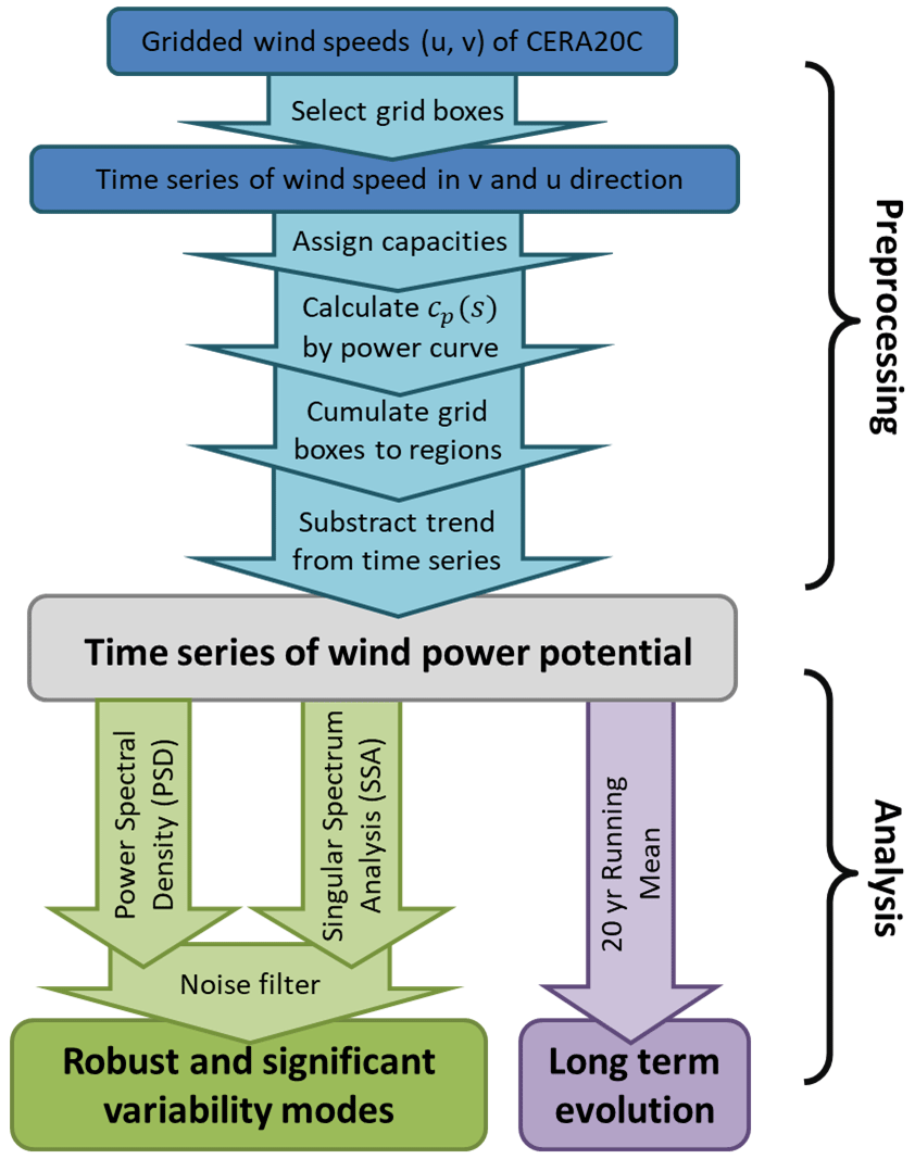
Figure 1 Flow chart of the main parts of the data processing. In the upper part the prepossessing from ECMWF product to wind power potential time series is shown (blue), in the lower part the different analysis tools and their products are shown (green and purple).

2.1 Power potential

We compute wind power potential from 1900 to 2010 over Europe based on the wind components (u, v) from the coupled reanalysis CERA-20C (ECMWF) at a height of 10 m. CERA-20C is an ensemble reanalysis consisting of 10 members with a spatial resolution of 1.125 ${}^{\circ }\times \mathrm{1.125}$ ^∘ and a temporal resolution of 3 h (Laloyaux et al., 2018). We use all ensemble members even though ensemble spread is limited.

As in Tobin et al. (2016), we assume a wind turbine hub height of 80 m and calculate hub height-wind speeds from 10 m wind components as

$$\begin{array}{}\text{(1)}& s\left(t\right)=\sqrt{u^{\mathrm{2}}\left(t\right)+v^{\mathrm{2}}\left(t\right)}({\displaystyle \frac{\mathrm{80}\text{m}}{\mathrm{10}\text{m}}}{)}^{\mathrm{1}/\mathrm{7}}.\end{array}$$

Wind power potential c_P is subsequently computed from the wind speed using a standard power curve (cf. Tobin et al., 2016) as

$$\begin{array}{}\text{(2)}& {\displaystyle }{c}_{\mathrm{P}}\left(s\right)=\left\{\begin{array}{ll}\mathrm{0}& \text{for }{s}_{\text{in}}>s\ge s_{\text{out}},\\ \frac{s^{\mathrm{3}}-s_{\text{in}}^{\mathrm{3}}}{s_{\text{r}}^{\mathrm{3}}{s}_{\text{in}}^{\mathrm{3}}}& \text{for }{s}_{\text{in}}\le s<s_{\text{r}},\\ \mathrm{1}& \text{for }{s}_{\text{r}}\le s<s_{\text{out}},\end{array}\right.\end{array}$$

assuming a cut-in velocity of s_in=3.5 m s⁻¹, a rated velocity of s_r=12 m s⁻¹ and a cut-out velocity of s_out=25 m s⁻¹. To isolate the effect of changes in resource availability, we leave the allocation of wind parks constant over the 20th century. In other words, we calculate the wind power potential during the twentieths century that could have been generated from a fixed wind park setup.

CERA-20C features strong upward trends in wind speeds, in particular over the oceans (Wohland et al., 2019b). The trends are linked to the assimilation of marine wind observations and are likely spurious. We therefore subtract the linear trend from the wind power potential time series as in Wohland et al. (2019a). It was shown before that multidecadal wind generation variability of CERA-20C, ERA-20C and 20CR is very similar after subtracting the linear trend at least in Germany (Wohland et al., 2019a), thus justifying the use of a single reanalyses in this particular case. All three centennial reanalyses also show the same relationship with multidecadal winter NAO variability, suggesting that the underlying physical processes are equally well captured in the de-trended data sets. Therefore, this study is based on CERA-20C only.

2.2 Definition of the regions

In the German North Sea we use real-world installed capacities from the Open Power System Database, totalling 4.5 GW (OPSD, 2018). Real world data is lacking for the Greek Mediterranean, hence we follow (Karanikolas et al., 2011) who provide plausible estimates of suitable wind park locations and sizes. Wind parks are distributed mainly over seven grid boxes in the Aegean and capacity totals at 8.3 GW. Short of real world data and good scenarios in the Portuguese Atlantic Coast, we utilize each grid box in the area 10.25–11.375^∘ W and 33.375–41.25^∘ N with turbines of 100 MW. As verified later on, the precise siting of the turbines has negligible impact on multidecadal generation characteristics (see Fig. 4), justifying the different approaches taken in different regions. In Sect. 3.2, we assume uniform capacities of 100 MW in each grid box as we seek to investigate generation variability independent of installed capacity.

2.3 Spectral analysis

To gain insight into the statistical properties of the time series, we use two methods to analyze their spectrum, namely the periodogram and singular spectrum analysis (SSA). Additionally we define a noise model to quantify the significance of spectral peaks.

2.3.1 Power spectral density

A periodogram shows the power spectral density (PSD) of a time series which is the squared Fourier transformed (Vaughan et al., 2011)

$$\begin{array}{}\text{(3)}& P_{xx}\left(\mathit{\nu }\right)={\displaystyle \frac{\mathrm{1}}{\mathrm{2}\mathit{\pi }N}}{\left|\sum _{n=\mathrm{0}}^{N-\mathrm{1}}{X}_n{e}^{-i\mathit{\nu }n\mathrm{\Delta }t}\right|}^{\mathrm{2}},\end{array}$$

where the power spectral density P_xx(ν) denotes the variance which occurs at a frequency ν for a time series with the values $\mathit{\{}{X}_n:\mathrm{0}\le n\le N\mathit{\}}$, length N and temporal resolution Δt.

As usual in real world time series, we expect the wind potential time series to be a superposition of several (periodic) signals and an underlying stochastic process. When investigating spectral properties, this means that the spectrum consists of several peaks plus background noise. The background together with effects of finite-length time series and non-sinusoidal signals complicates the identification of real signals. A test for statistical significance is therefore needed and we introduce a noise model in the following to which we apply a χ²-test to quantify the significance of single peaks.

2.3.2 Noise model

White or red noise is often assumed for the background signal in atmospheric time series analysis. The auto-regressive process of order 1 (AR(1) process) is the simplest statistical model for a red noise time series (Mann and Lees, 1996). We therefore choose an AR(1) reference process $Y_t={\mathrm{\Phi }}_{\mathrm{1}}{Y}_{t-\mathrm{1}}+{\mathit{ϵ}}_t$ to model red noise contribution of the original time series X_t. The coefficients Φ₁ and ϵ_t are obtained by the Yule-Walker equations (Kirchgässner et al., 2012, p. 49–51) and fully determine the process (see Appendix A1 for details).

2.3.3 Singular spectrum analysis

Singular spectrum analysis (SSA) decomposes a signal in its eigenmodes and is particularly well suited for relatively short and noise time series as the wind potential time series we assess. Shortness is to be understood relative to the investigated time periods of multiple decades. Furthermore SSA enables detection of non-sinusoidal signals in contrast to Fourier transformed based analysis since the generating function is not restricted to sinusoidal functions. The decomposition is achieved by solving the eigenproblem of the signal's correlation matrix. Our approach follows Ghil et al. (2002) where the application of SSA is demonstrated for the Southern Oscillation Index. For consistency, we also normalize the time series by its standard deviation. To focus on long-term variability, we mute higher frequency variability, including the seasonal cycle, by resampling from 3 h to annual values. The window size M is set to 50 years due to the limited sample size of N=110 in line with Ghil et al. (2002) suggestion to avoid the hard limit of $N/M<\mathrm{1}$. This reduces the outcomes of SSA to modes with periods smaller than M (Vautard et al., 1992). We choose the singular value decomposition (SVD) estimate (Broomhead and King, 1986) to calculate the correlation matrix C_X (see Appendix A2 for detailed revision).

Diagonalizing C_X yields the eigenvalues $\mathit{\{}{\mathit{\lambda }}_k:\mathrm{1}\le k\le M\mathit{\}}$ which are ranked in decreasing order ${\mathit{\lambda }}_{\mathrm{1}}\ge {\mathit{\lambda }}_{\mathrm{2}}\ge \mathrm{\dots }\ge {\mathit{\lambda }}_N\ge \mathrm{0}$. Each eigenvalue λ_k of C_X corresponds to the variance of the time series in the direction of the corresponding eigenvector ρ_k, also known as empirical orthogonal functions or EOFs.

Ghil et al. (2002) also give a noise filtering method for SSA reported as Monte Carlo SSA (MC-SSA): Basically we apply SSA to 1000 synthetic time series {Y_t} that were generated by the noise model, in our case it is the AR(1) process (see Appendix A3). For each synthetic time series, we calculate the correlation matrix C_Y using SVD and project it onto the eigenvectors ρ_k of the real data. Thus each diagonal entry of the projected matrices is a surrogate of the corresponding eigenvalue λ_k of the real data. Eigenvalues within the inner 90 % of the surrogates are rejected as noise, eigenvalues out of this range are reported as significant signals.

2.4 20 year running mean

Our spectral analysis is complemented by analysing the long term evolution of wind power potential. Therefore we take the 20-year running mean of the time series. By averaging over 20 years, high-frequency variability is eliminated and the long-term evolution can be assessed. This provides a good proxy for lifetime energy generation since 20 years roughly correspond to wind turbine life times.

We define a 20-year forward running mean as

$$\begin{array}{}\text{(4)}& G_{\mathrm{20}}\left(t\right)=\sum _{t^{\prime }=t}^{t+\mathrm{20}\text{ year}}G\left(t^{\prime }\right),\end{array}$$

where G(t) denotes the detrended time series and G₂₀(t) is the 20-year running mean covering the period of 1900 to 1990. Extension beyond 1990 (i.e., mean from 1990 to 2009) is impossible due to data availability. The seasonal potential ($G_{\mathrm{20}}^{\text{season}}\left(t\right)$) is calculated analougously by using the seasonal time series instead.

2.5 North Atlantic Oscillation

Following Wohland et al. (2019a) we compare winter North Atlantic Oscillation (NAO) with the long term evolution. This yields further insight into the relation of local wind power potential to the general circulation of the atmosphere. The NAO dominates climate variability in the North Atlantic sector, particular in winter, affecting weather as well as climate allover Europe (Marshall et al., 2001). We refer here to it as the first principle component of sea-level pressure over the area 20–80^∘ N and 90^∘ W – 40^∘ E as detailed in Omrani et al. (2016). Our NAO index is computed from sea-level pressure data from the Hadley Center (Rayner et al., 2003) over the winter months December, January and February.

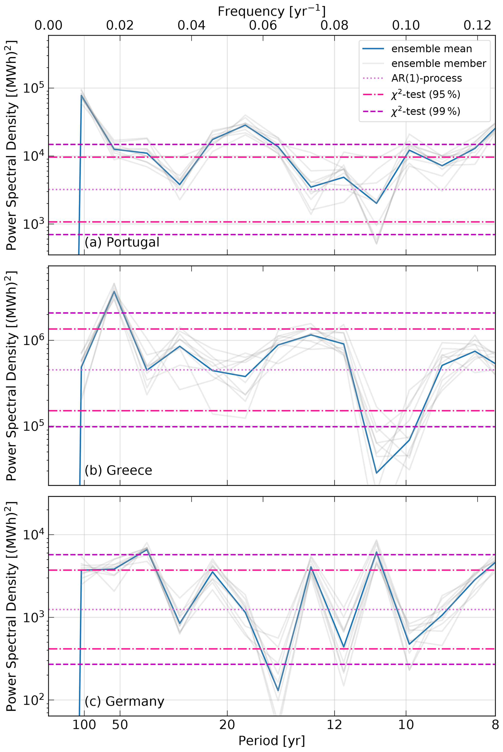
Figure 2 Wind power potential spectra of three locations in Europe. Each panel shows the PSD for offshore wind power potential in the 20th century (blue denotes ensemble mean, gray ensemble members) in a multi-decadal range: (a) Portuguese Atlantic Coast, (b) Greek Mediterranean, (c) German North Sea. An AR(1)-process models the noise and an applied χ²-test gives confidence intervals of 95 % (dashed) and 99 % (dash-dotted).

3 Results

3.1 Spectral analysis reveals multi-decadal variability

We show the PSD for three separated regions of Europe, namely (a) the Portuguese Atlantic Coast, (b) the Greek Mediterranean and (c) the German North Sea (see Fig. 2). All three reveal significant peaks on multi-decadal timescales. The strongest peaks occur in Portugal where the periods $P_{\mathrm{1}}^{\text{POR}}\approx \mathrm{100}$ year and $P_{\mathrm{2}}^{\text{POR}}\approx \mathrm{20}$ year are statistically significant at the 99 % level. A third peak is visible around P≈8 years but will not be studied here as we focus on multi-decadal peaks. While only one 99 % significant peak exists for the Greek Mediterranean ($P_{\mathrm{1}}^{\text{GRE}}\approx \mathrm{50}\mathrm{years}$), there are two for the German North Sea ($P_{\mathrm{1}}^{\text{GER}}\approx \mathrm{45}\mathrm{years}$ and $P_{\mathrm{2}}^{\text{GER}}\approx \mathrm{10}\mathrm{years}$). In other words, multi-decadal variability is a large scale phenomenon that impacts different parts of Europe differently.

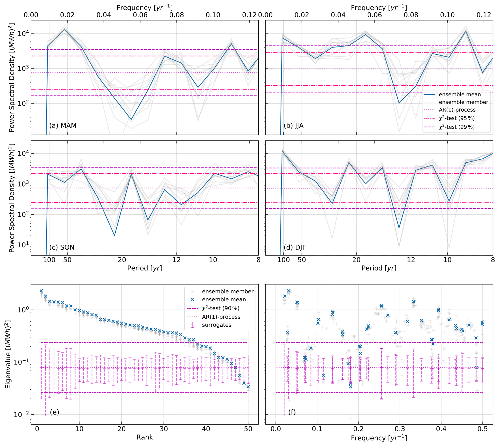
Figure 3 Spectra of wind power potential for Portuguese Atlantic Coast. The panels (a)–(d) show the PSD of each season (blue denotes ensemble mean, gray ensemble members). The confidence level of 95 % (dashed) and 99 % (dash-dotted) is given. The panels (e) and (f) show the eigenspectrum of SSA (blue denotes ensemble mean, gray ensemble members). Eigenvalues are ordered by rank in (e) and by frequency in (f) with confidence interval given by the inner 90 % of the surrogates and a χ²-test (90 %).

We investigate the evolution in all regions in more detail which provides further evidence for the existence of multi-decadal peaks. Focusing on the seasonal evolution in Portugal, the peaks of seasonal PSD (see Fig. 3a–d) support the periods $P_{\mathrm{1}}^{\text{POR}}$ and $P_{\mathrm{2}}^{\text{POR}}$. The PSD of summer (b) and winter (d) both show peaks at $P_{\mathrm{1}}^{\text{POR}}$ and $P_{\mathrm{2}}^{\text{POR}}$. In spring (a), we observe a mode with period P^POR≈50 years which might be a harmonic of $P_{\mathrm{1}}^{\text{POR}}$. In winter another significant peak occurs with a period $P_{\mathrm{3}}^{\text{POR}}\approx \mathrm{11}$ years which is not mirrored in the annual values. The PSD of autumn (c) shows no peaks that are significant at the 99 % level but there is one which exceeds the 95 % significance threshold P≈30 years.

In addition, we report the eigenspectrum of the SSA for Portuguese Atlantic Coast. In Fig. 3e the eigenvalues (EV) are ordered by their rank and in (f) by the frequency of the belonging EOF. The structure of the eigenvalues in (e) show three groups formed by gaps and different slopes. The first six form a group that carries a large part of the variance (≈33 %) despite the small group size and is therefore of higher interest than the second group (7th–14th EV ≈26 % of total variance) or the last group (15th–34th EV ≈33 % of total variance). Lower eigenvalues (rank > 34) are indistinguishable from noise and consequently rejected by the noise hypothesis, which is represented by the surrogates and a χ²-test, providing another reason to focus on high eigenvalues. A closer look to the frequency ordered EVs (f) shows that the first and second EV correspond to the frequency ν₁=0.031–0.022 yr⁻¹ (P≈30–45 years) and the fifth and sixth to the frequency ${\mathit{\nu }}_{\mathrm{2}}=\mathrm{0.052}{\mathrm{yr}}^{-\mathrm{1}}$ (P≈20 years). While the latter matches perfectly with $P_{\mathrm{2}}^{\text{POR}}$, the former hardly fits $P_{\mathrm{1}}^{\text{POR}}$. This lacking fit is a consequence of the resolvable frequencies in SSA because a window size of M=50 years restricts the EOFs to frequencies $\mathit{\nu }\ge \mathrm{0.02}{\mathrm{yr}}^{-\mathrm{1}}$. The first and second EV consequently correspond to the lowest resolvable frequency, further validating variability on very long time scales. Moreover, P≈30–45 years agrees well with the seasonal PSD results in spring and winter (see Fig. 3a) and autumn (see Fig. 3c). The third and fourth EV correspond to a relatively high frequency $\mathit{\nu }=\mathrm{0.333}{\mathrm{yr}}^{-\mathrm{1}}$ (P≈3 years) and therefore do not contribute to multi-decadal variability.

SSA of German North Sea and Greek Mediterranean confirm the reported periods of PSD as well (see Supplement Figs. S1 and S2). We have refrained from a detailed analysis of these sites in favour of a more detailed discussion of their interconnections, because we focus on balancing potential.

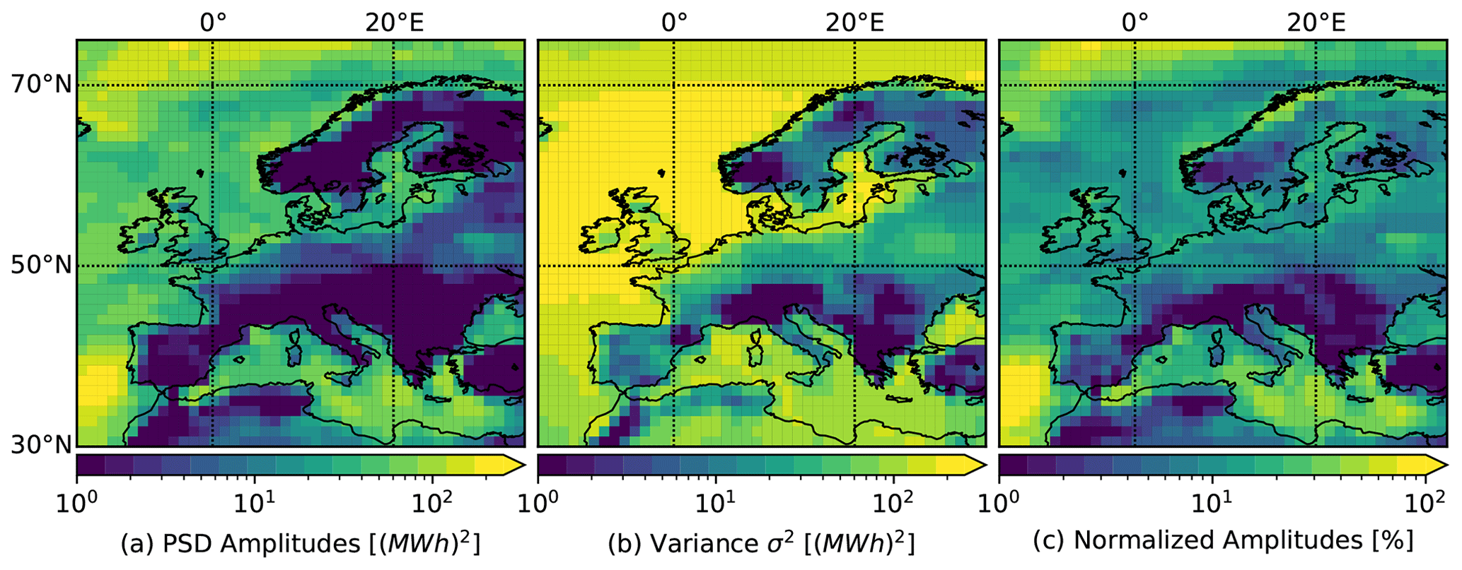
Figure 4 Analysis of multi-decadal peaks in the PSD for each grid point in Europe. (a) The maximum amplitude for multi-decadal timescales ν<0.1 yr⁻¹ in comparison to (b) the 3-hourly variance σ². (c) The ratio of maximal amplitude and variance give the normalized amplitude. The shown signals are significant for a 90 % confidence level at least.

3.2 Significant multi-decadal peaks everywhere across Europe

Whether or not multi-decadal variability affects large areas determines its system-wide relevance. A PSD investigation reveals the existence of at least one significant multi-decadal peak in every grid box in Europe (see Fig. 4). We show in (a) a map of the maximal amplitude in the multi-decadal range for each grid box, additionally we give in (b) the variance of the full time series and in (c) the ratio of both as normalized amplitude. The normalized amplitude quantifies the relative importance of multi-decadal variability and short term variability. In (a) the amplitudes located offshore are particularly high in contrast to those onshore. This clear demarcation of offshore and onshore areas weakens in the normalized amplitudes (c) because high amplitudes coincide with high variances in some areas (e.g., the North Sea). Both, amplitude and normalized amplitude, host a maximum in the Portuguese Atlantic coast (around 250 MWh²). The amplitudes in the German North Sea are lower (around 50 MWh²), and the high variance there is leading to even lower normalized amplitudes. In the Mediterranean isolated higher amplitudes (around 100 MWh²) are shown as around the Greek islands in the Aegis. Due to moderate variance in the Mediterranean, the normalized amplitudes reveal isolated areas of medium height there, too. In order to ensure comparability between the locations, we have assumed the same capacity (100 MW) for each grid box in this investigation. This distinguishes the amplitudes here from those shown in Fig. 2 for Greek Mediterranean and German North Sea, where we use capacities of installed or planed power plants (see Sect. 2.2).

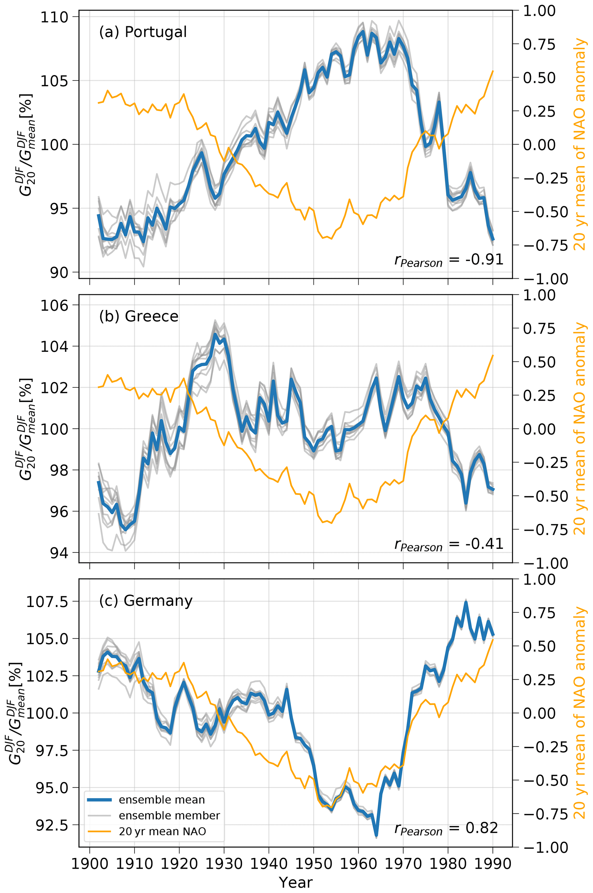
Figure 5 Normalized 20 year running mean in relation to the NAO anomaly. Blue denotes the normalized 20 year running mean of wind power generation potential in DJF of the ensemble mean (grey denotes same for each ensemble member) at three different locations: (a) Portuguese Atlantic Coast, (b) Greek Mediterranean, (c) German North Sea. Yellow lines show the 20-year running mean of the NAO anomaly.

3.3 Timing of multi-decadal variability differs vastly throughout Europe

The 20-year mean confirms that offshore wind power potential in Portuguese Atlantic Coast, Greek Mediterranean and German North Sea show a similar period in multi-decadal variability. Nevertheless, their timing differs vastly (see Fig. 5 for the normalized running mean of winter and Fig. 6 for the annual values). All three panels in Fig. 5 show multi-decadal variability with an amplitude of ±6 %–10 % reaching maxima and minima at least once over the last century. The peaks and dips, however, do not occur simultaneously: While Portugal shows 8 % above average potential in 1960, Germany is 7 % below average at the same time (a, c). In fact, the long-term evolution in Portugal is inverse to the evolution in Germany. This similarity strongly suggest a common dynamical origin by a larger climate pattern. This common forcing could be the NAO as high negative/positive correlations of 20-year mean NAO and Portuguese/German wind power illustrate ($\text{r}=-\mathrm{0.91}$ and r=0.82, respectively). The link between NAO and wind potential is less pronounced in Greece (see Fig. 5b), likely because local and regional effects play a more important role in Greece compared to large-scale atmospheric variability over the North Atlantic region.

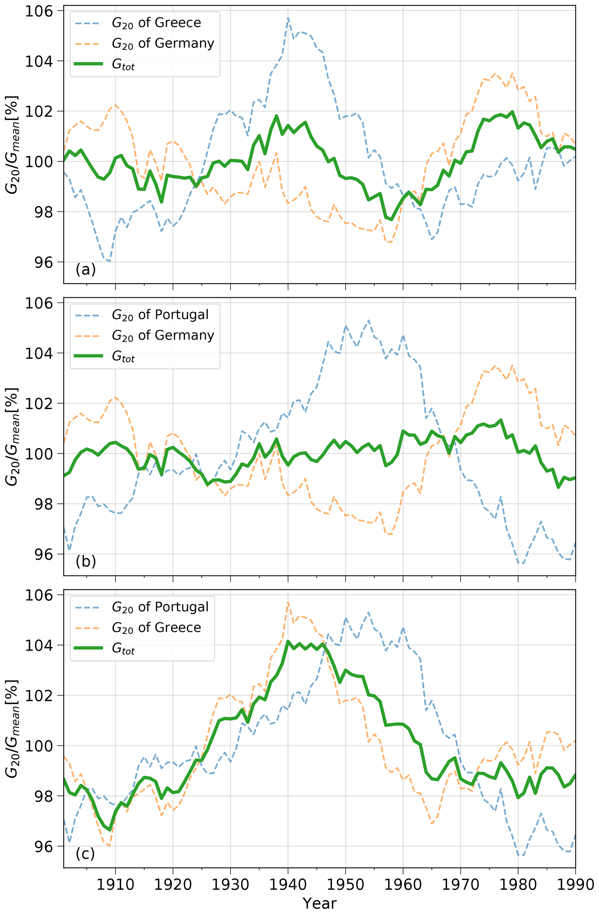
Figure 6 Pairwise combination of 20 year running mean of three locations. The corresponding location of the 20 year running mean (dashed blue and yellow) is given in the legend of each panel. The variance of their combined 20 year running mean G_tot (green) is minimized in (a) by λ_opt=0.42, in (b) by λ_opt=0.39 and in (c) by λ_opt=0.36.

3.4 Different multi-decadal evolution allows for efficient balancing

The pronounced timing differences between wind power potential in the individual countries and their relation to the NAO suggests capability for spatial balancing. To study the positive effects from combining potential in different countries through inter country transmission, we define the total potential (G_tot) of wind turbines in two countries as

$$\begin{array}{}\text{(5)}& G_{\text{tot}}(t,\mathit{\lambda })=\mathit{\lambda }{G}_{\mathrm{1}}\left(t\right)+(\mathrm{1}-\mathit{\lambda })G_{\mathrm{2}}\left(t\right),\end{array}$$

where $\mathit{\lambda }\in [\mathrm{0},\mathrm{1}]$ is a mixing parameter that describes the share of wind parks installed in country 1 and G_1,2(t) is the 20-year running mean potential in the countries 1 and 2, respectively. A simple minimization of the variance of G_tot yields an optimum mixing λ_opt. Figure 6 shows total potential G_tot using λ_opt and the potential of the individual countries G_1,2. The total potential of the combinations in (a) and (b) has distinctly smaller variance than the potential of single locations (by a factor of 3–10). In contrast, combining Greece and Portugal (c) leaves the variance essentially unchanged. These different effects on variance can be conceptually understood: Assuming comparable values for the variances of both locations $\text{Var}\left(G_{\mathrm{1}}\right(t\left)\right)\approx \text{Var}\left(G_{\mathrm{2}}\right(t\left)\right)\approx \text{Var}\left(G_{\mathrm{1},\mathrm{2}}\right(t\left)\right)$ and the optimal values of λ being of the order of $\mathrm{1}/\mathrm{2}$ (${\mathit{\lambda }}_{\text{opt}}\approx \mathrm{1}/\mathrm{2}$), the total variance is reduced to:

$$\begin{array}{}\text{(6)}& \begin{array}{rl}\text{Var}\left(G_{\text{tot}}\right(t,{\mathit{\lambda }}_{\text{opt}}& \approx \mathrm{1}/\mathrm{2}\left)\right)\approx {\displaystyle \frac{\mathrm{1}}{\mathrm{2}}}\text{Var}\left(G_{\mathrm{1},\mathrm{2}}\right(t\left)\right)\\ & +{\displaystyle \frac{\mathrm{1}}{\mathrm{2}}}\text{Cov}\left(G_{\mathrm{1}}\right(t),G_{\mathrm{2}}(t\left)\right).\end{array}\end{array}$$

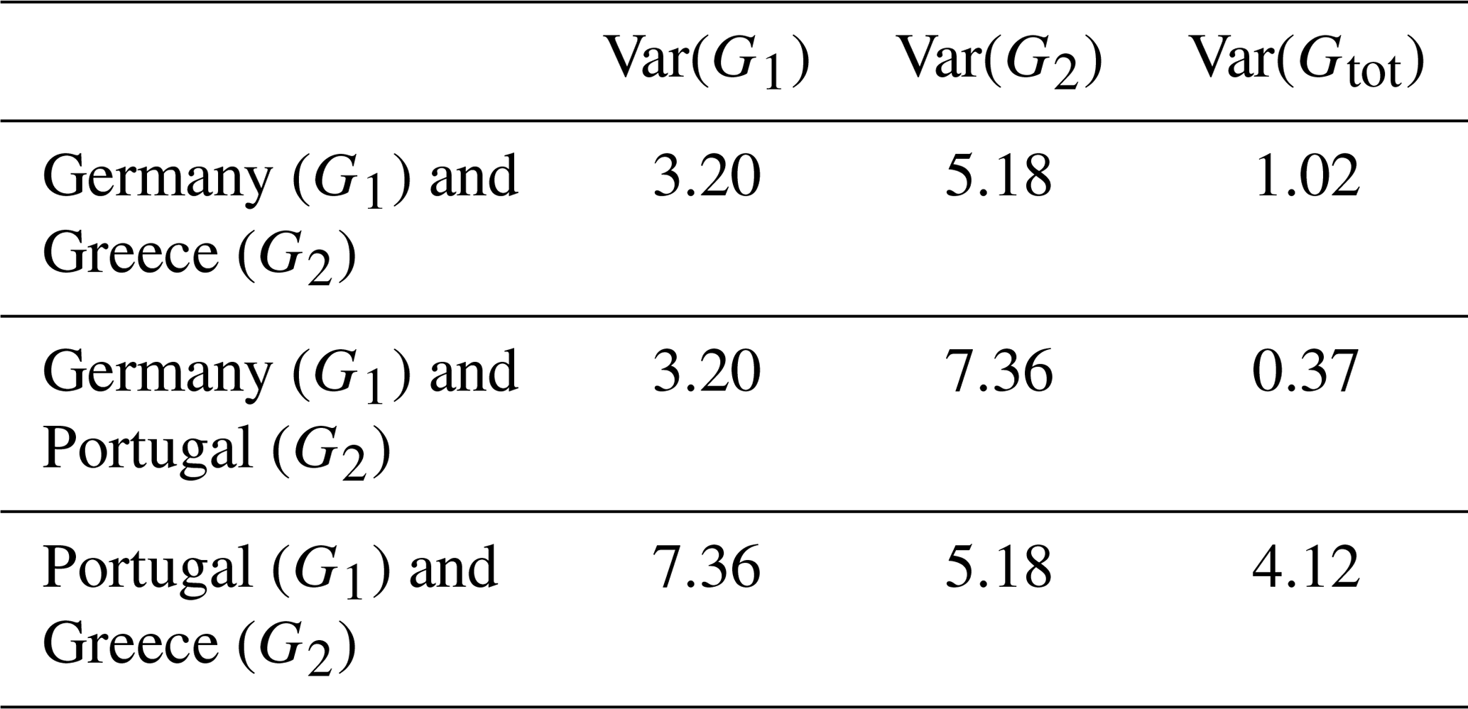
The values of Var(G_1,2(t)) and Var(G_tot(t,λ_opt)) are given in Table 1 respectively for the combinations shown in Fig. 6.

The introduced metric in Eq. (6) means that the effectiveness of the variability mitigation depends on the sign of the co-variance. If the combined 20-year running mean variance is higher than half of the individual variances, the co-variance is positive and reinforces the joint variance. This is true for combining Portuguese and Greek potential (see Table 1), where joint variance is higher than half of Portuguese or Greek variance. However, if the joint variance is smaller than half of the 20-year running mean variance, which is correct for balancing between for Greece and Germany as well as for Portugal and Germany (see Table 1), the co-variance is negative thus balancing is effective. The joint variance of Portugal and Germany is a magnitude lower than the variance in Germany. The joint variance of Greece and Germany is significantly lower than half of Var(G_Ger) as well. However, the benefit through balancing of Germany and Portugal is substantially higher in comparison.

Table 1 Variances of each location (Var(G_1,2)) and their combinations (Var(G_tot)) as shown in Fig. 6.

4 Conclusions

Using a state-of-the art centennial coupled ocean-atmosphere reanalysis, CERA20C, and correcting for likely spurious trends due to marine wind speed assimilation, we report significant multi-decadal offshore wind potential variability in Portugal, Greece and Germany. Our results are robust to the chosen statistical approach as Power Spectral Density, Singular Spectrum Analysis and visual inspection of long-term time series reveal consistent results. Portuguese and German multi-decadal wind power evolution are strongly coupled with the NAO in winter but with different signs. This emphasises mitigation potential through inter-county transmission.

In particular, we report two significant multi-decadal modes at the Portuguese Atlantic Coast indicated by significant peaks at periods of $P_{\mathrm{1}}^{\text{POR}}=\mathrm{50}$–100 years and $P_{\mathrm{2}}^{\text{POR}}=\mathrm{15}$–20. They occur consistently in both spectral methods. We report similar modes in the Greek Mediterranean ($P_{\mathrm{1}}^{\text{GRE}}=\mathrm{50}\mathrm{years}$) and the German North Sea (with $P_{\mathrm{1}}^{\text{GER}}=\mathrm{45}$ and $P_{\mathrm{2}}^{\text{GER}}=\mathrm{10}\mathrm{years}$). Moreover, we demonstrate the existence of significant multi-decadal modes all over Europe, which are connected to slowly varying climate patterns, such as the NAO.

The long-term development of offshore wind potential shows strong differences, especially between North and South Europe. While the German offshore potential correlates strongly with NAO (r=0.82), the Portuguese and Greek anti correlate ($r=-\mathrm{0.91}$ and $r=-\mathrm{0.41}$, respectively). Furthermore, Portuguese multi-decadal wind power evolution is inverse to German evolution: a positive NAO leads to above average potential in Portugal and below average potential in Germany (each by around 7 %). These differences allow mitigation of multi-decadal variability through spatial balancing. In particular, we uncover that combining Portuguese and German offshore potential reduces multi-decadal fluctuations around the mean value from ±5 % to only about ±1 %. Combining Germany and Greece also results in a reduction of variability but only to around ±2 %. In contrast, combining locations in Portugal and Greece yields no reduction. Our research therefore suggest that multi-decadal wind power variability can be tackled with optimized wind park allocation and inter-country transmission, methods that were proved effective at synoptic scales (Grams et al., 2017; Rodriguez et al., 2014). At the same time, local solutions to balance generation variability, such as storage (Tröndle et al., 2019), will most likely fail to deliver on multi-decadal timescales. Inter-country transmission is therefore a promising approach for future fully renewable power systems because it allows stable supply despite multi-decadal resource fluctuations.

Appendix A: Details to methods

A1 Auto-regressive process

In general an auto-regressive processes (AR(p)) of order p could approximate an original time series X_t by a stochastic process Y_t defined by

$$\begin{array}{}\text{(A1)}& Y_t={\mathit{ϵ}}_t+\sum _{i=\mathrm{1}}^p{\mathrm{\Phi }}_i{Y}_{t-i},\end{array}$$

where Φ_i are fixed coefficients which characterize the deterministic process and ϵ_t is a sample drawn from a Gaussian distribution with zero mean and variance σ² (Percival and Walden, 1993). Note that an AR(p) process is special case of an AR(p+1) process, where ${\mathrm{\Phi }}_{p+\mathrm{1}}=\mathrm{0}$. In our spectral analysis an AR(1) process estimates the underlying red noise. Thus estimating Φ₁ an σ² fully determine the process. The corresponding power spectral density S_Y(ν) of Y_t is the Fourier transformed lag-l auto co-variance γ_l given as,

$$\begin{array}{}\text{(A2)}& S_Y\left(\mathit{\nu }\right)=\sum _{l=-\mathrm{\infty }}^{\mathrm{\infty }}{\mathit{\gamma }}_l{e}^{-\mathrm{2}\mathit{\pi }i\mathit{\nu }l}={\displaystyle \frac{{\mathit{\sigma }}^{\mathrm{2}}}{\mathrm{1}-{\mathrm{\Phi }}_{\mathrm{1}}\mathrm{2}\cos \left(\mathrm{2}\mathit{\pi }\mathit{\nu }\right)+{\mathrm{\Phi }}_{\mathrm{1}}}}.\end{array}$$

The parameters σ² and Φ₁ are obtained by the Yule-Walker equations (Kirchgässner et al., 2012, p. 49–51). For p=1 they simplify to

$$\begin{array}{}\text{(A3)}& {\mathit{\gamma }}_{\mathrm{0}}={\displaystyle \frac{{\mathit{\sigma }}^{\mathrm{2}}}{\mathrm{1}-{\mathrm{\Phi }}_{\mathrm{1}}^{\mathrm{2}}}}{\mathit{\gamma }}_l={\displaystyle \frac{{\mathit{\sigma }}^{\mathrm{2}}{\mathrm{\Phi }}_{\mathrm{1}}^{\mathrm{|}l\mathrm{|}}}{\mathrm{1}-{\mathrm{\Phi }}_{\mathrm{1}}^{\mathrm{2}}}},\end{array}$$

where γ₀ and γ₁ are the auto co-variances of the time series with lag zero and one.

A2 SVD approach

Following Broomhead and King (1986), the SVD estimates C_X from the trajectory matrix D. The rows of D are the $N^{\prime }=N-M+\mathrm{1}$ lagged M-dimensional vectors $\mathit{\{}{\stackrel{\mathrm{̃}}{\mathit{X}}}_t=(X_t,X_{t+\mathrm{1}}$, …, $X_{t+M-\mathrm{1}}):t=\mathrm{1}$, …, $N-M+\mathrm{1}\mathit{\}}$ of length M given by sliding a window of size M over the time series. In particular D is given by

$$\begin{array}{}\text{(A4)}& {\displaystyle }\mathbf{D}=\left(\begin{array}{cccc}{X}_{\mathrm{1}}& X_{\mathrm{2}}& \mathrm{\cdots }& X_M\\ X_{\mathrm{2}}& X_{\mathrm{3}}& \mathrm{\cdots }& X_{M+\mathrm{1}}\\ \mathrm{⋮}& \mathrm{⋮}& \mathrm{\ddots }& \mathrm{⋮}\\ X_{N-M+\mathrm{1}}& X_{N-M+\mathrm{2}}& \mathrm{\cdots }& X_N\\ ,\end{array}\right)\end{array}$$

and C_X is defined as

$$\begin{array}{}\text{(A5)}& {\mathbf{C}}_X={\displaystyle \frac{\mathrm{1}}{N^{\prime }}}{\mathbf{DD}}^{\mathrm{T}},\end{array}$$

where the superscript T denotes the transpose of a matrix.

A3 MC-SSA

As suggested in Ghil (1997), we construct a time series using the stochastic process of the chosen noise model (here AR(1)-process with the parameters given by the Yule-Walker equation $Y_t={\mathrm{\Phi }}_{\mathrm{1}}{Y}_{t-\mathrm{1}}+{\mathit{ϵ}}_t$) and project this to the eigenstates of the signal with the SVD approach. This is done by first calculating the correlation matrix C_Y of the surrogate time series Y_t as shown in Eq. (A2). And second by multiply with the eigenvectors {ρ_k} of the original process X_t to the right and left of C_Y :

$$\begin{array}{}\text{(A6)}& \mathbf{\Delta }=\text{diag}\left(\begin{array}{ccc}({\mathit{\rho }}_{\mathrm{1}}& \mathrm{\cdots }& {\mathit{\rho }}_M)\end{array}{\mathbf{C}}_Y{\begin{array}{ccc}({\mathit{\rho }}_{\mathrm{1}}& \mathrm{\cdots }& {\mathit{\rho }}_M)\end{array}}^T\right).\end{array}$$

Each element of Δ is a surrogate Δ_i corresponding to an eigenvalue λ_i. This projection is repeated 1000 times generating 1000 surrogates per eigenvalue derived from the same noise hypothesis.