 | 04 Mar 2020
Assessment of local covariance estimation through Least Squares Collocation over Iran
Sabah Ramouz
Yosra Afrasteh
Mirko Reguzzoni
Abdolreza Safari
Covariance determination as the heart of Least Squares Collocation gravity field modeling is based on fitting an analytical covariance to the empirical covariance, which is stemmed from gravimetric data. The main objective of this study is to process different local covariance strategies over four regions with different topography and spatial data distribution in Iran. For this purpose, Least Squares Collocation based on Remove – Compute – Restore technique is implemented. In the Remove step, gravity reduction in regions with a denser distribution and a rougher topography is more effective. In the Compute step, the assessment of the Collocation estimates on the gravity anomaly control points illustrates that data density is more relevant than topography roughness to have a good covariance determination. Moreover, among the different attempts of localizing the covariance estimation, a recursive approach correcting the covariance parameters based on the agreement between Least Squares Collocation estimates and control points shows better performance. Furthermore, we could see that covariance localization in a region with sparse or bad distributed observations is a challenging task and may not necessarily improve the Collocation gravity modeling. Indeed, the geometrical fitness of the empirical and analytical covariances – which is usually a qualitative test to verify the precision of the covariance determination – is not always an adequate criterion.
- Article
(6313 KB) - Full-text XML
- BibTeX
- EndNote


Least Squares Collocation (LSC) takes root on both deterministic and stochastic modeling. This is an advantage that makes LSC a flexible apparatus in the gravity field determination. Basically, it consists of two steps. First, the deterministic part of the signal is removed from the data, in case estimating it by a least squares adjustment. Second, residuals are modelled in a stochastic way and the noise is filtered out by minimizing the mean square estimation error. Moreover, the capability of combining heterogeneous observations as well as the possibility of predicting quantities that are different from the observed ones are other advantages of LSC (Moritz, 1980; Sansò, 1986). In gravity field modeling, LSC is usually implemented through the Remove – Compute – Restore (RCR) technique. This means that the systematic parts of the gravity signal related to the global and topographical effects are first removed and then restored after applying the LSC estimation on the gravity residuals (Sansò and Sideris, 2013).
One of the most critical task in LSC gravity field modeling is the covariance (COV) determination. Tscherning and Rapp (1974) introduced a harmonic 3D COV model (TR1974) for the gravity anomaly Δg:
where rP and rQ are the radii of the Earth at the points P and Q, RE is the mean radius of the Earth which is assumed to be equal to 6371 km, N is the maximum degree of the global gravity model (GGM) that is removed from the data, Pℓ is the Legendre polynomial of degree ℓ, ψ is a spherical distance between points P and Q, and is the error degree variance of the reference GGM coefficients. The first term of the right hand side of Eq. (1) is devoted to model the error of removing long wavelengths of the signal through the RCR technique. The second term is written in such a way that the summation can be expressed in a closed form and therefore can be numerically evaluated (Tscherning and Rapp, 1974, pp. 43–45). In case of block-mean values, the expression for the covariance model also includes the smoothing factors βℓ (Rapp, 1977):
In this work the available data are point-wise and Eq. (1) is used for the computations. TR1974 is a harmonic 3D COV model and, in contrast to 2D COV models which work on a sphere, it takes the radii of the observations into consideration. This property is relevant in our case studies due to the rough topography in Iran (see Sect. 2). Note that the TR1974 3D COV model depends on the spherical distance between gravimetric observations, as well as their radii.
The three unknown variables α (scale factor of the GGM global error variance), A (scale factor of the residual signal variance at higher degrees), and the Bjerhammer radius RB are estimated by fitting TR1974 to the Empirical COV (E_COV) computed from the available local observations. In this approach, homogeneity (2D position-independency) and isotropy (azimuth-independency) have to be presumed to compute the E_COV, albeit these assumptions are not applicable in everywhere of the Earth gravity field. To overcome these limitations, there have been some attempts in mathematical geodesy. Tscherning (1999) used Riesz-representer to account for anisotropy of the COV determination, Barzaghi et al. (2001) presented a new idea for the estimation of a non-homogeneous local COV. Moreover, Keller (2002) and Kotsakis (2007) made use of wavelet applications in non-homogeneous COV estimation, and Darbeheshti and Featherstone (2009) introduced kernel convolution to improve COV determination, even though none of these attempts could attain the wide generality of the TR1974 approach. Another limitation is that the radii of the observations are ignored when computing the empirical covariance, that is fitted by the model in Eq. (1) assuming .
Ramouz et al. (2019) used the LSC method based on TR1974 for gravity field modeling in Iran which led to the best geoid model for the region in the sense of Standard Deviation (SD) of the difference between the model and the GNSS/Leveling geoid values. They implemented two strategies for the COV determination; the former used all terrestrial observations in a uniform COV model (U_COV), the latter divided the region into four subareas and then determined the COV model of each subarea independently (P_COV). The effect of these two strategies on the LSC algorithm showed that, at least in this case study, localization of the COV modeling resulted in a slightly better accuracy. In Ramouz et al. (2019), the heterogeneity and the lack of data in some parts of Iran lay at the root of the simplicity in the localization and region subdivision performed in their work. It is expected that the localized COV determination, if it is implemented in a more appropriate way based on the region characteristics, will guide us to a better gravity field modeling via LSC.
In this research, various criteria in the COV determination are investigated. The effect of the observation spatial distribution and the topography roughness on the data reduction in RCR, the refinement of the observation spatial distribution to smooth its pattern and improve the COV determination, the implementation of different COV strategies and also the sensitivity analysis of the COV localization to the observation spatial distribution are studied. In the next section, the properties of the regions and the gravimetric data are introduced, also explaining how the data reduction is implemented. In Sect. 3, the process of the COV modeling is described and various attempts for the COV determination in the regions are tested and evaluated. Finally, in Sect. 4 the results of the research are discussed and a conclusion is drawn.
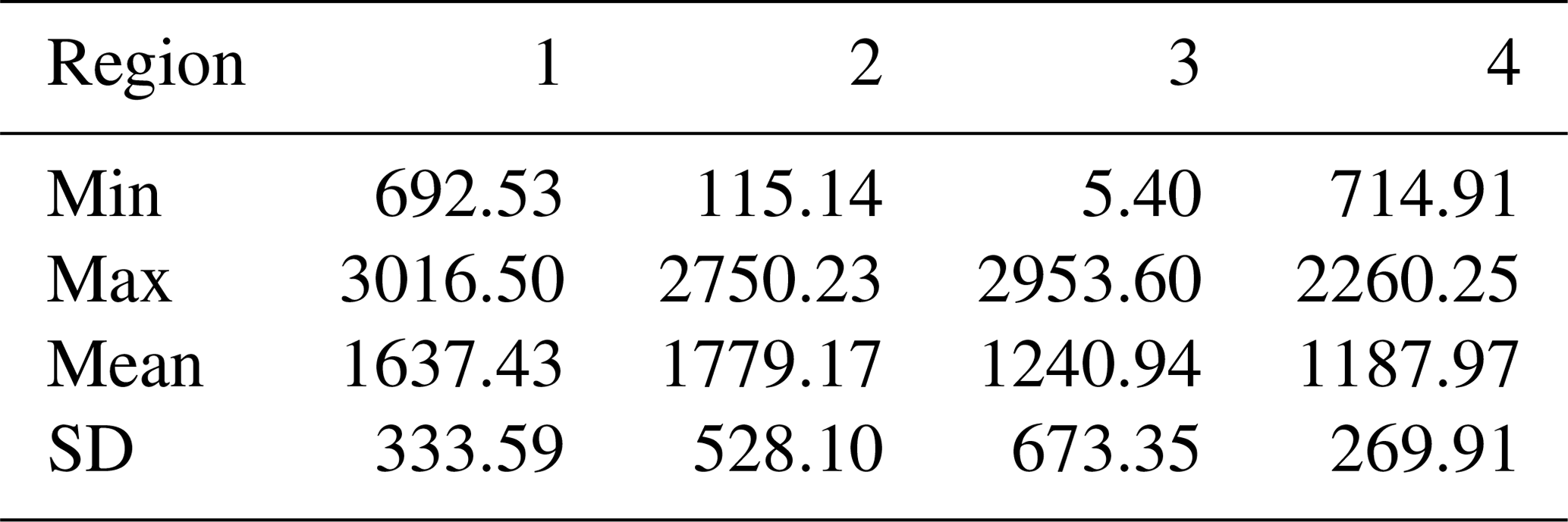
Four regions with a size of 2.5×3 arcdeg with different characteristics were chosen in Iran. First and third regions (R1 and R3) have approximately 5 arcmin network resolution (Fig. 1 and Table 1). Note that R1 has a relatively smoother topography than R3 (see Table 2). Second and fourth regions (R2 and R4) have approximately 13 arcmin network resolution. In this case, R2 has a relatively rougher topography than R4. The free air gravity anomalies are collected from terrestrial observations of zeroth, first, second, and third order gravity networks, with mean uncertainties of 0.001, 0.010, 0.015, and 0.020 mGal respectively. Moreover, free air gravity observations from a first order precise leveling network (PLN) with a mean uncertainty of about 0.050 mGal were included (Saadat et al., 2018). In R1 and R3, almost all the observations are from PLN and third order network, while PLN and second order network observations embody the majority of R2 and R4 (Fig. 2).
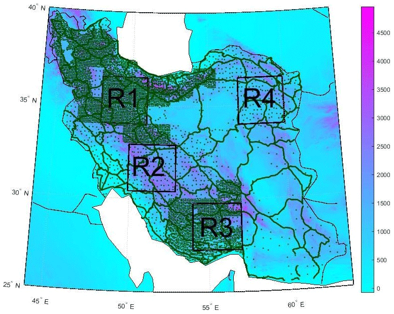
Figure 1Distribution of gravity data over Iran (green dots). Topography as background (m).
Table 1Location of each region based on geographical coordinates and corresponding number of observations.

According to the RCR technique, residual gravity anomalies are obtained by
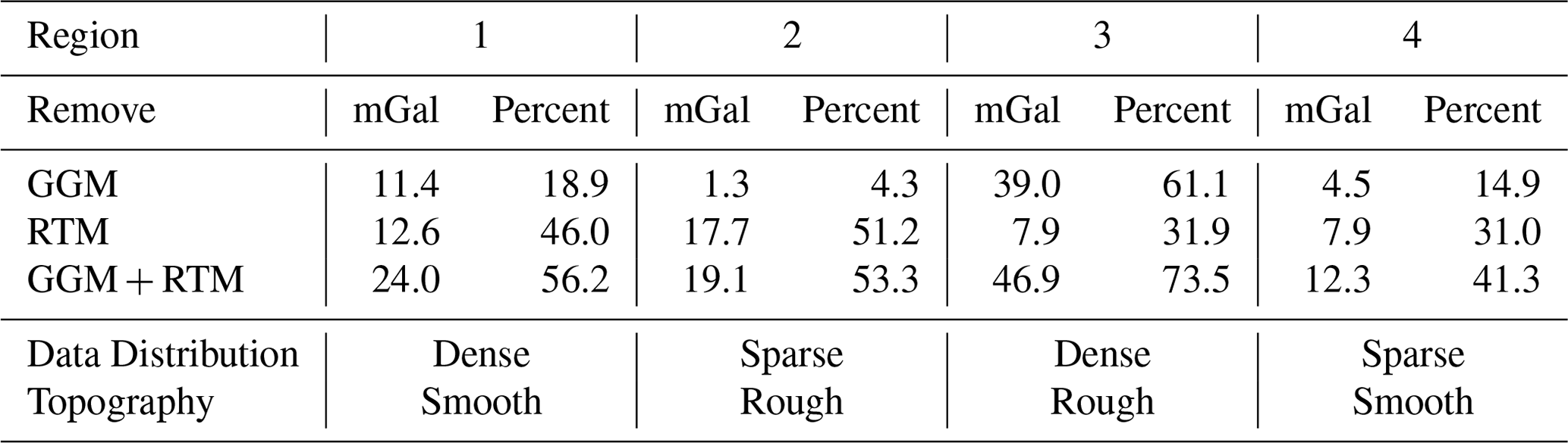
where ΔgFA is the free-air gravity anomaly, ΔgGGM is the long wavelength of the gravity signal derived from a GGM and ΔgRTM is the residual terrain model (RTM) effect. To remove ΔgGGM from the observations, EIGEN6C4 (Förste et al., 2014) up to degree and order 360 was used, as it was shown that EIGEN6C4 has better performance than other GGMs in Iran (Foroughi et al., 2017). Moreover, to remove ΔgRTM, a residual terrain modeling technique (Forsberg, 1984) with the SRTM1′′ (NASA, 2013) digital elevation model (DEM) was used in the same way of Ramouz et al. (2019). A reference grid of 0.5∘ resolution, corresponding to degree and order 360 of the GGM effect, was derived from SRTM1′′ and used as a mean elevation surface in order to remove the long-wavelengths of the topographic gravity signal. Moreover, inner and outer zone cap-radius (r1 and r2) were chosen equal to 13 and 80 km, respectively (Forsberg, 1984). As it is shown in Tables 3 and 4, the GGM and RTM effects represent a significant part of the gravity signal in these regions. On average, 28.3 % of the SD of the gravity anomalies was removed by the GGM and 31.2 % of the remaining SD by the RTM technique. Altogether, the removed effects in these four regions are about 59.5 % of the original signal. Apart from R3 where there is a considerable reduction from the GGM, RTM effects are generally more significant in these regions. Again in Table 4, the regions are classified based on data spatial distribution and topographic pattern. It comes out that removing a systematic part of the signal in denser regions (R1 and R3) is more effective. In addition, statistics in Table 4 reveal that in the regions with rougher topography (R2 and R3) reductions have more impact compared to the regions with a similar data spatial distribution. It should be noted that the density of the data distribution has more influence on the reductions than the topography roughness.
Table 3Statistics of gravity anomalies before and after removing GGM and RTM effects (mGal).
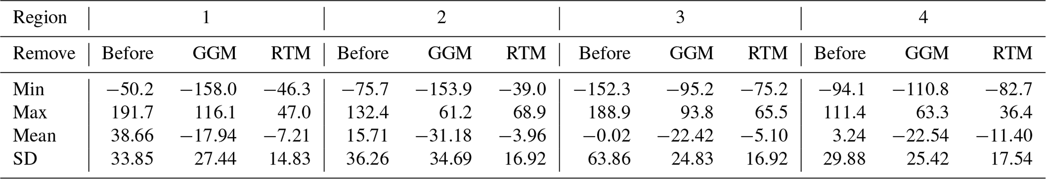
Table 4Percentage of removing GGM and RTM effects on the SD of the gravity signal in each region.
To assess the quality of the COV estimation, residual gravity anomalies from Eq. (3) for each region were partitioned into two sub-sets: observations and control data. To this aim, R1 and R3 were tiled to a set of 7×7 arcmin windows, and R2 and R4 to 14×14 arcmin windows. Then, every window was sequentially selected and alternately classified as observations or control data (Fig. 2). It should be noted that, at the edge of each region, control points were excluded in a strip of 15 arcmin thickness. In other words, this means that output data are limited to a 2×2.5 arcdeg region, though input data spread over the 2.5×3 arcdeg area.
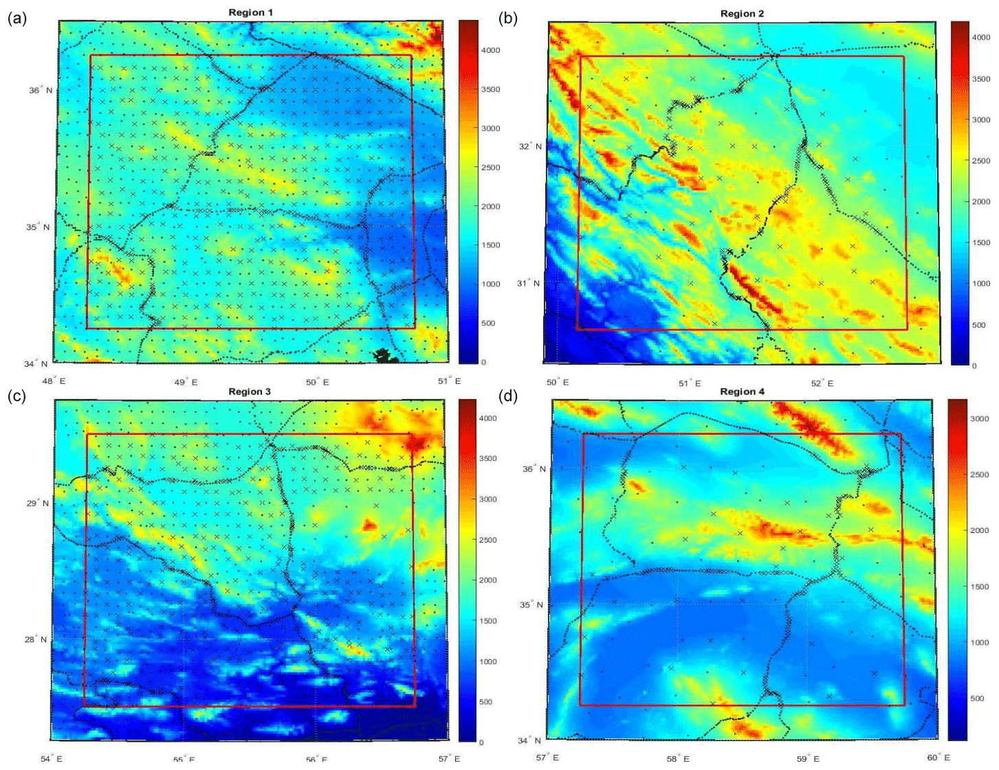
Figure 2Divided data into observations (dots) and control points (crosses) in the regions (a) R1, (b) R2, (c) R3 and (d) R4. Topography as background (m).
3.1 Covariance estimation
In this section, the implemented procedure for the COV estimation using TR1974 COV model is described. First, the E_COV is computed by using the following estimator:
where and are the ith and jth residual gravity anomalies with a spherical distance ψij falling in the interval
Δψ is the so-called Sample Interval (SI), which should be proportional to the overall spatial resolution of the data in the region. The selected SI values for these four regions are reported in Table 5. These values could be compared to the data distribution in Fig. 2. By SI in hand, the E_COV of each region was computed and the two parameters of the E_COV, namely the covariance at zero distance (ψ=0) or variance (C0) and the correlation distance (ξ), i.e. the spherical distance where the value of covariance becomes half the value of C0, were determined (Table 5).
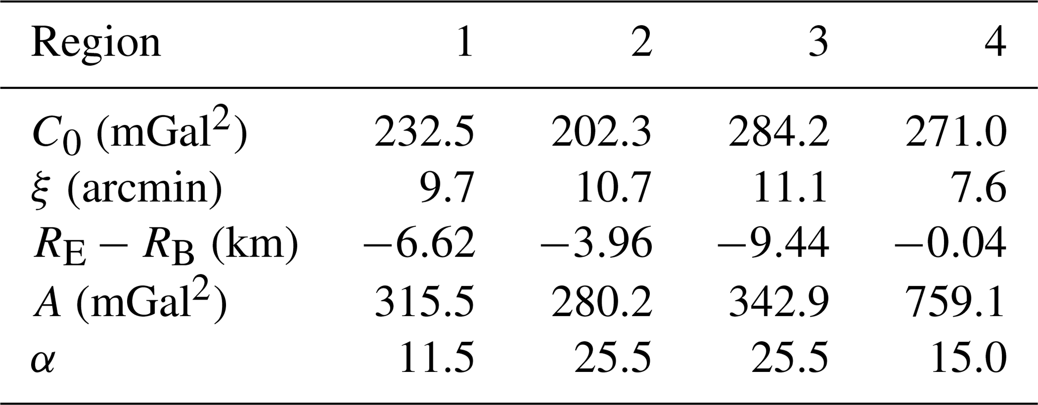
After that, an Analytical COV (A_COV) has to be modeled by fitting the E_COV in the best way. This analytical formula was determined by estimating the three parameters (depth to the Bjerhammer sphere (RE−RB), A and α) in Eq. (1) through a least squares adjustment implemented in the COVFIT software (Knudsen, 1987). The A_COV is predicted with a given spherical distance step, that is named Mean Data Spacing (MDS). In the same way as SI for E_COV, the chosen value of the MDS depends on the data spatial resolution (Table 5). The estimated A_COV parameters are included in Table 5. In Fig. 3, the E_COV and its fitted A_COV model are illustrated for each region.
Table 5Parameters of the empirical and analytical COVs in each region.

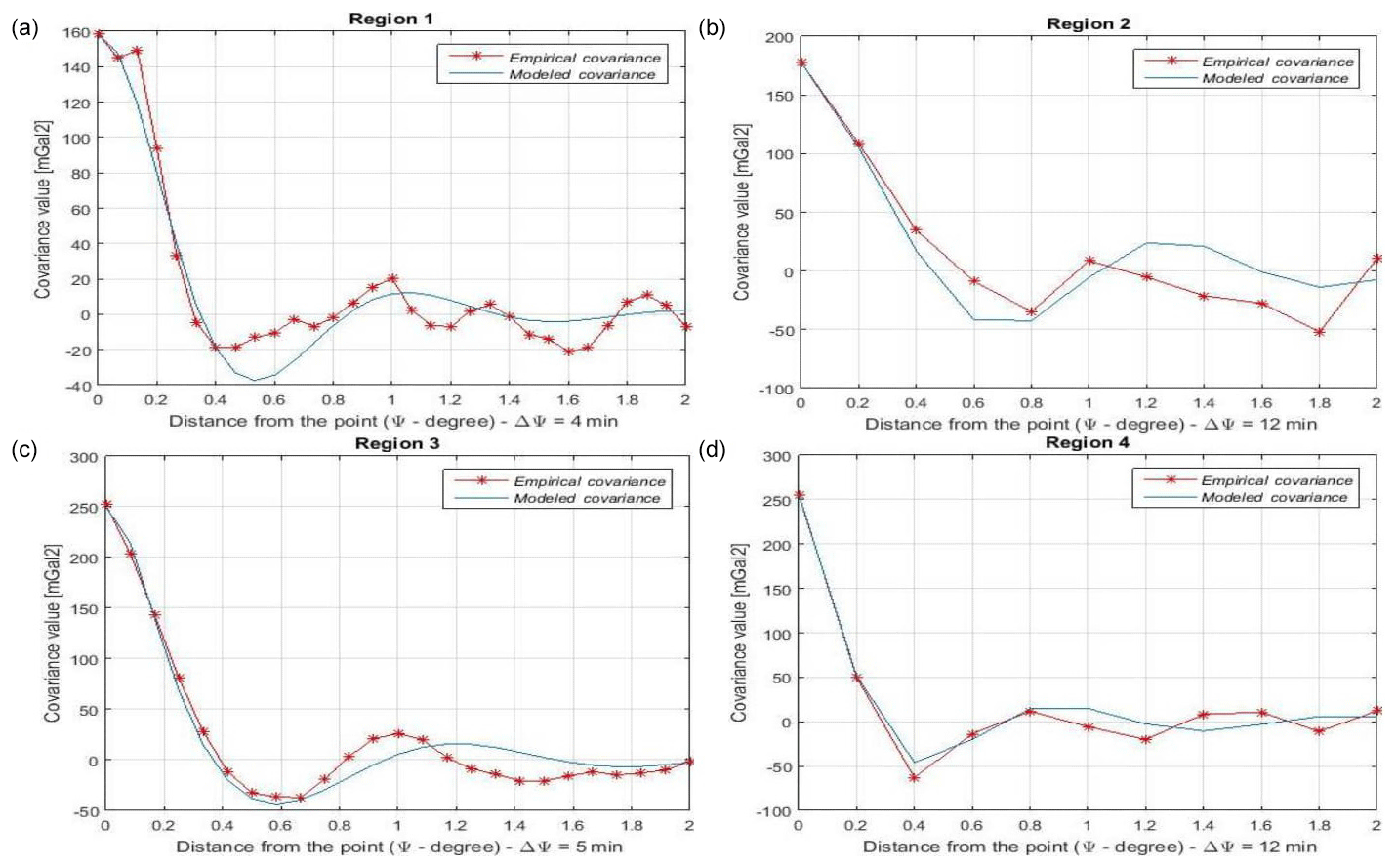
Figure 3Empirical and fitted COV for residual gravity anomalies of the regions (a) R1, (b) R2, (c) R3 and (d) R4.
3.2 Refinement of gravity data distribution
The quite rough E_COV in Fig. 3 and their modeled A_COV, which did not fit the E_COV adequately, encouraged us to check if a refinement of the data distribution can improve the COV determination. To this aim, data were decimated by using a minimum-distance criterion. That to say, all the observations with distances less than 1.5 arcmin in R1 and R3 and 2 arcmin in R2 and R4 to the targeted observation were removed, thus reducing the print of the heavily linear crowded PLN observations (Fig. 4). The number of the observations and control data before and after the distribution refinement are shown in Table 6, and the COV parameters for the four regions in Table 7. Note that SI and MDS values are the same as in Table 5. As one can see from Fig. 5, this attempt geometrically improves the COV fitting.

Figure 4Observations (dots) and control points (crosses) in the regions (a) R1, (b) R2, (c) R3 and (d) R4 after refining the data distribution. Topography as background (m).

Figure 5Empirical and fitted COV for the regions (a) R1, (b) R2, (c) R3 and (d) R4 after refining the data distribution.
Table 6Number of observations and control points before and after the data distribution refinement in each region.
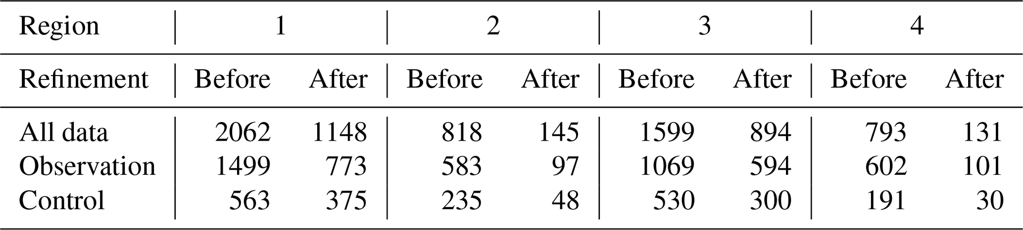
Table 7Parameters of the empirical and analytical COVs after the data distribution refinement in each region.
3.3 Assessment of covariance estimation
In the previous section, the effect of the spatial distribution refinement of the datasets was visually assessed by comparing the fitness between empirical E_COV and estimated A_COV. Here, we will statistically evaluate it by computing the LSC output at control points. For this purpose, LSC gravity field modeling has to be implemented on the datasets. To perform the LSC procedure, besides the estimation of the COV parameters that has been described in Sect. 3.1 and 3.2, the observation and control subsets were respectively used as input and output of the LSC process in each region. In Table 8, the results of LSC modeling accuracy with respect to control data are shown for U_COV, P_COV, Simple local COV (S_COV) and Refined local COV (R_COV) solutions. Because of using localized observation datasets, as well as P_COV, S_COV and R_COV are categorized into local COV strategies. Note that P_COV and S_COV are computed in the same way but they refer to areas with a different size. The difference between S_COV and R_COV is not in the area size, but in the number of used data, since for the R_COV computation the data distribution refinement described in Sect. 3.2 is performed. To estimate the LSC uniform and partial solutions, the related COV parameters are taken from Ramouz et al. (2019), while in the case of the LSC simple and refined solutions, the COV parameters are reported in Tables 5 and 7, respectively.
Table 8Accuracy of the LSC gravity estimation based on uniform, partial and local COVs modeling in each region (mGal).
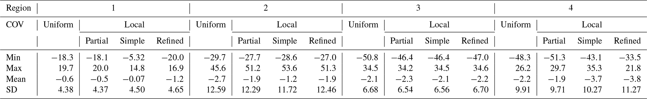
At the first glance, Table 8 shows that, irrespective of the processing strategy, a good spatial data distribution has a positive effect on the COV determination and LSC gravity modeling. That is to say, the accuracy of the LSC models in R1 and R3 is better than R2 and R4 at control points. On the other hand, the topography roughness has a reverse effect. Note that R1 and R4 have better accuracy than R3 and R2 at control points, respectively in the case of dense and sparse data distribution regions. In fact, both R1 and R4 have a relatively smoother topography pattern.
As was expected from Ramouz et al. (2019), P_COV has slightly better performance than U_COV over the case study regions. On the other hand, S_COV which is spatially more localized than P_COV could not reduce the SD of the differences over all the regions, but it could only decrease the mean of the differences. Table 8 also illustrates that, even though the fitness between E_COVs and A_COVs is enhanced after the data distribution refinement, the accuracy of the LSC modeling by applying R_COV is deteriorated in our case studies. This result confirms the claim of Paciorek (2003), who had mentioned that fitting E_COV to A_COV may not give reliable estimates. The statistics information of Table 8 shows that localization of the COV determination is a difficult task and does not necessarily lead to an improvement for the output of the LSC. One can see that the localized COV determination in R2 and R3 with relatively rough topography is positive or at least not damaging, while it seems to negatively work in R1 and R4. Note that the improvement in R2 with sparse data distribution is more than in the case of the dense distributed R3.
3.4 Attempt to improve covariance determination
Another idea to analyze the influence of the local COV estimation on the LSC gravity modeling was to improve the estimation of the TR1974 covariance parameters by means of a recursive LSC procedure. In order to implement this idea, S_COV parameters are used as the initial values for this Improved local COV (I_COV) strategy. In the first step, LSC gravity anomaly estimation is performed at the location of control points using S_COV parameters. In the second step, the best ratio between the two parameters A and α is determined in such a way that mean and SD of the differences between LSC outputs and control data get minimum. In the next step, (RE−RB) is changed and LSC estimation is repeated at the same control points. This process has to be continued until these differences reach their minimum values. In Table 9, the final values for I_COV parameters in each region are shown.
Table 9Parameters of the improved local COV modeling in each region.
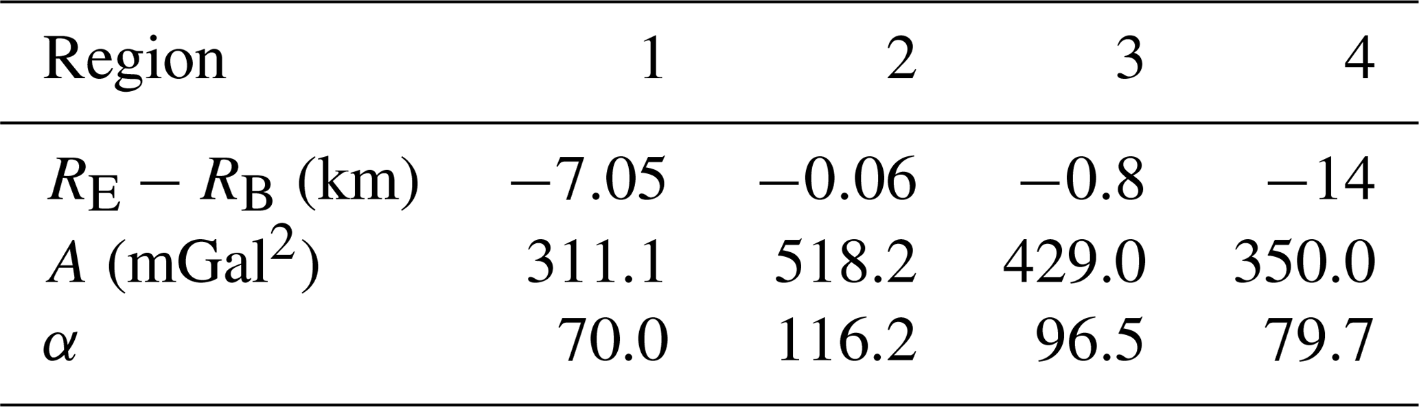
Table 10Accuracy of the LSC gravity estimation based on the improved local COV modeling in each region (mGal).
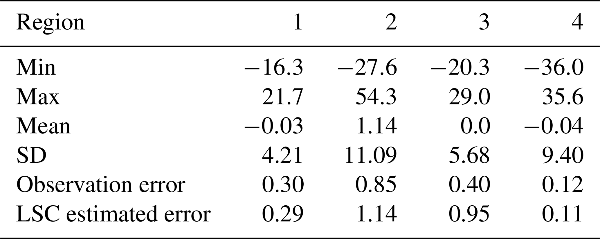
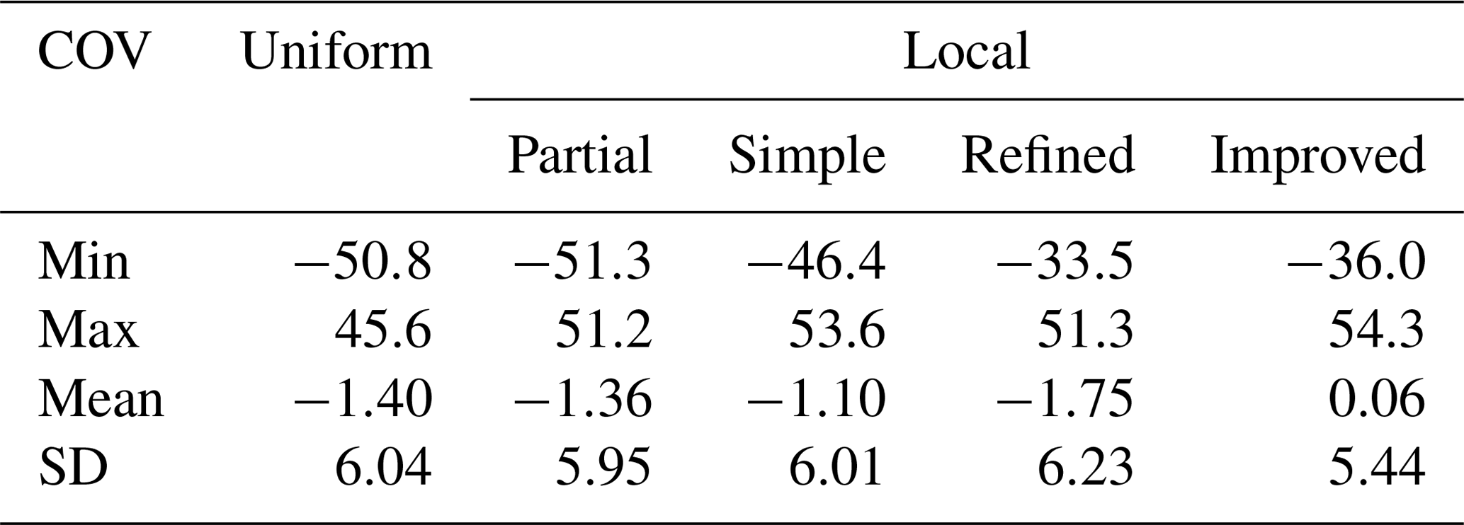
In comparison with the results of the above-mentioned strategies, I_COV shows an improvement in terms of SD and especially in removing systematical effects in the differences with control points (Table 10). Considering all regions, I_COV estimation approach reduces mean and SD of the results by 96 % and 10.2 %, respectively (Table 11). The values of the parameter α in I_COV are significantly different from the corresponding values of the other COV strategies in all regions. Based on the information of Tables 5 and 7, α ranges between 0 to 39, while for I_COV it is between 70 and 116 (Table 9).
Table 11Statistics of the different COV strategies over all the regions (mGal).
3.5 Sensitivity of the localization and covariance parameters analysis
Improvement of LSC modeling through COV localization was one of the main objectives of this study. Therefore, we examined different covariance estimation strategies besides the one presented in Ramouz et al. (2019). A considerable outcome of this comparison and analysis was the sensitivity of COV localization to the spatial data distribution in our case study. That is, COV localization in a region with sparse data distribution, like R2 and R4, is more challenging than in a dense one. In other words, precise local COV determination in sparse or bad data distributed regions is a difficult task that requires to accurately estimate the COV parameters. It means that a small change in the input parameters results in a big deviation in the output model. This is detectable in Table 12, where the variance of the mean and SD values of the different LSC solutions at control points in each region is depicted. In R2 and R4 the variations of both mean and SD statistics of the LSC modeling are much more than R1 and R3.
Table 12Sensitivity of the LSC solutions with respect to their data distribution and topography roughness (mGal2).
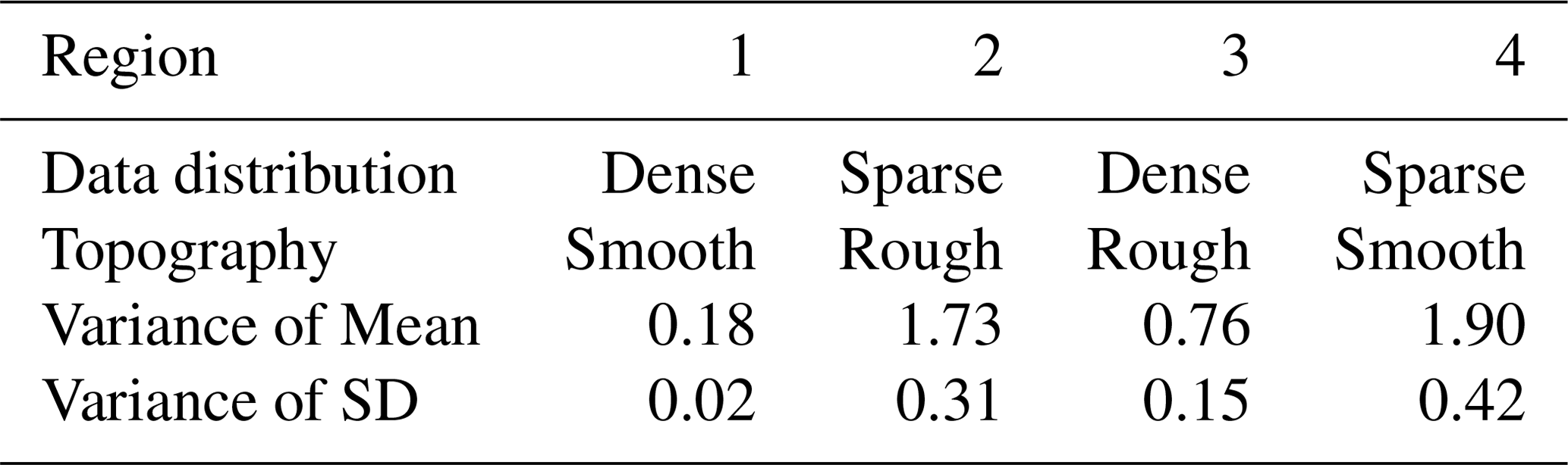
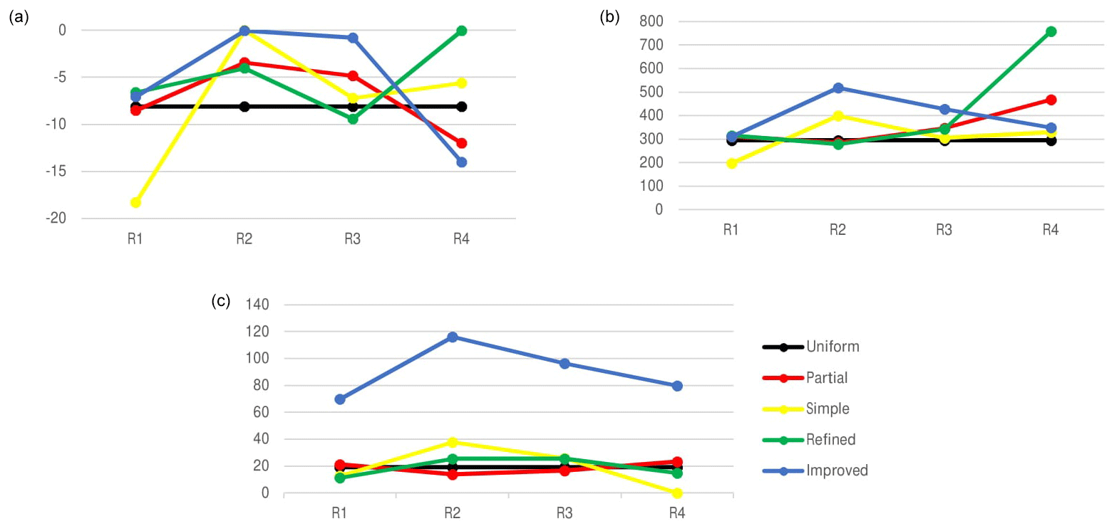
Figure 6COV parameters of the different strategies in each region: (a) RE−RB (km), (b) A (mGal2), and (c) α.
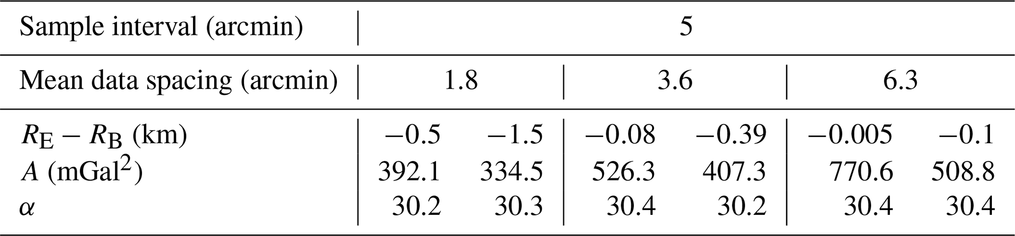
Table 13Sensitivity of the outputs of Refined COV estimation in the region R2.
We also studied the changes in the COV parameters of the four regions with their different topography and spatial observations distribution. In Fig. 6, the COV parameters for each region are depicted based on the different COV strategies. According to the three graphs of the COV parameters, the behaviour of I_COV is more similar to the one of S_COV, although there is a shift of about 70 units between values of S_COV and I_COV strategies for the parameter α. Actually, the assessment of α requires more in-deep investigations. Combined GGMs suffer from the lack of accurate terrestrial observations in Iran. Furthermore, previous studies showed that combined GGMs cannot model the gravity field in Iran as well as in Europe (for instance, Amjadiparvar et al., 2011; Foroughi et al., 2017; Kiamehr, 2009). Therefore, whereas LSC gravity modeling has been done in France by α=2.05, α≅0 for R4 could not be a precise estimation (Yildiz et al., 2012).
As was mentioned in Sect. 3.1, the SI for E_COV and MDS for A_COV could be defined based on the region data distribution. But, when the data are not distributed well in the case study, choosing an appropriate SI turns to a hard job. For example, SI usually should be set to less than the minimum distance between the observations, but this is impossible in our regions, because of the presence of highly dense PLN observations before data refinement. In this case, different values for SI and especially MDS should be tried to find the best one. In addition, MDS affects convergence of the adjustment. That is to say, the velocity of the adjustment convergence is proportional to the chosen MDS. With a bigger MDS, the adjustment converges sooner. Moreover, when the MDS is small, sometimes the adjustment (specifically RE−RB) does not converge, or converges to different values of the parameters. For this situation, the adjustment becomes sensitive to the initial values which by various quantities lead to different outputs. As an example, the COV estimation for R2 is showed in Table 13, when using different initial values.
Data distribution itself is a challenging element that could affect the adjustment convergence. In R2 and R4 (before data refinement), for all the SI values and all the MDS values from 0.5 to 13 arcmin, the estimation of RE−RB is sensitive to the initial value.
In this study, our focus was on the localization and enhancement of the COV determination through LSC gravity modeling in Iran. For this purpose, in addition to U_COV and P_COV strategies, three localized attempts named S_COV, R_COV and I_COV were also investigated. First, four regions with different characteristics were chosen to analyze the gravity reduction and it was concluded that the data reduction based on the RCR technique in a dense distributed region is more influential. More precisely, in R1 and R3 averagely 65 % of the gravity anomaly signal is reduced, while in R2 and R4 this number is about 47 %. Moreover, one can find a relation between the region topography pattern and the data reduction. Between R1 and R3, the reduction in R3 which has relatively rougher topography is more effective, as well as the reduction in R2 between the sparser distributed regions R2 and R4.
Naturally, non-homogeneous data distribution led to rugged E_COV functions, and necessarily, the A_COV function could not fit the E_COV in an optimal way. By refining the data distribution, we obtained smoother E_COV and consequently better fitted A_COV. The impact of the data distribution refinement on the LSC modeling was investigated, showing that despite of the visual analysis of the consistency between E_COV and A_COV, refining the data distribution could not enhance the accuracy of LSC solutions with respect to the gravity anomaly control points in the regions. Therefore, the geometrical fitness of the E_COV and A_COV, which is usually a test to verify the precision of the COV determination, is not an appropriate or at least an adequate criterion.
In spite of topography roughness, density of the data distribution has a positive effect on the COV determination and LSC gravity modeling. That is to say, the accuracy of the LSC models in R1 and R3 is better than R2 and R4 with respect to control points. Among various attempts for localization, the I_COV strategy shows better performance which could reduce mean and SD values of the differences between LSC model and control data, on average by 96 % and 10 % respectively. Moreover, the COV determination in a region is sensitive to the data distribution. Indeed, when the region has sparse or bad distributed data, the COV determination will turn to a challenging task and using local COV strategies may not necessarily improve the LSC gravity modeling.
It is necessary to mention that the findings of this study should be examined in other case studies with different geographical characteristics and spatial data distribution. Furthermore, the non-homogeneity and anisotropic properties of these regions and their effects on LSC modeling should be considered. Finally, future researches should certainly further test whether the I_COV approach could have the same performance on the GNSS/Leveling-derived geoid height as control points.
Both datasets (terrestrial gravity anomalies and GNSS/Leveling) are provided and processed by the National Cartographic Center (NCC) of Iran. Restrictions apply to the availability of these data, which were used under license for the current study, and so are not publicly available.
SR and YA conceived the idea, SR performed the computations and wrote the manuscript, YA and MR revised the manuscript, MR and AS supervised the findings of this work. All authors discussed the results and contributed to the final manuscript.
The authors declare that they have no conflict of interest.
This article is part of the special issue “European Geosciences Union General Assembly 2019, EGU Geodesy Division Sessions G1.1, G2.4, G2.6, G3.1, G4.4, and G5.2”. It is a result of the EGU General Assembly 2019, Vienna, Austria, 7–12 April 2019.
This paper was edited by Petr Holota and reviewed by two anonymous referees.
Amjadiparvar, B., Sideris, M. G., Rangelova, E., and Ardalan, A. A.: Evaluation of GOCE Based Global Gravity Field Models in Iran, presented at American Geophysical Union, Fall Meeting 2011, San Francisco, California, USA, 2011.
Barzaghi, R., Borghi, A., and Sona, G.: New Covariance Models for Local Applications of Collocation, in: IV Hotine-Marussi Symposium on Mathematical Geodesy, edited by: Benciolini, B., IAG Symposia, Springer, Berlin, Heidelberg, 122, 91–101, https://doi.org/10.1007/978-3-642-56677-6_15, 2001.
Darbeheshti, N. and Featherstone, W. E.: Non-stationary covariance function modelling in 2D least-squares collocation, J. Geod., 83, 495–508, https://doi.org/10.1007/s00190-008-0267-0, 2009.
Foroughi, I., Afrasteh, Y., Ramouz, S., and Safari, A.: Local evaluation of Earth Gravitational Models, case study: Iran, Geodesy Cartogr. 43, 1–13, https://doi.org/10.3846/20296991.2017.1299839, 2017.
Forsberg, R.: A Study of Terrain Reductions, Density Anomalies and Geophysical Inversion Methods in Gravity Field Modelling, Report 355, Department of Geodetic Science and Surveying, The Ohio State University, Columbus, 1984.
Förste, C., Bruinsma, S., Abrikosov, O., Lemoine, J. M., Marty, J. C., Flechtner, F., Balmino, G., Barthelmes, F., and Biancale, R.: EIGEN-6C4 The latest combined global gravity field model including GOCE data up to degree and order 2190 of GFZ Potsdam and GRGS Toulouse, GFZ Data Services, https://doi.org/10.5880/icgem.2015.1, 2014.
Keller, W.: A Wavelet Solution to 1D Non-Stationary Collocation with Extension to the 2D Case, in: Gravity, Geoid and Geodynamics 2000, edited by: Sideris, M. G., IAG Symposia, Springer, Berlin, Heidelberg, 123, 79–84, https://doi.org/10.1007/978-3-662-04827-6_13, 2002.
Kiamehr, R.: Evaluation of the New Earth Gravitational Model (EGM2008) in Iran, presented at European Geosciences Union General Assembly 2009, Vienna, Austria, 2009.
Knudsen, P.: Estimation and modelling of the local empirical covariance function using gravity and satellite altimeter data, B. Geod., 61, 145–160, https://doi.org/10.1007/BF02521264, 1987.
Kotsakis, C.: Least-squares collocation with covariance-matching constraints, J. Geod., 81, 661–677, https://doi.org/10.1007/s00190-007-0133-5, 2007.
Moritz, H.: Advanced Physical Geodesy, Herbert Wichmann Verlag, Karlsruhe, 1980.
NASA: NASA Shuttle Radar Topography Mission Global 1 arc second, Data set, NASA LP DAAC, https://doi.org/10.5067/measures/srtm/srtmgl1.003, 2013.
Paciorek, C. J.: Nonstationary Gaussian Processes for Regression and Spatial Modelling, PhD thesis, Carnegie Mellon University, Pittsburgh, USA, 2003.
Ramouz, S., Afrasteh, Y., Reguzzoni, M., Safari, A., and Saadat, A.: IRG2018: A regional geoid model in Iran using Least Squares Collocation, Studia Geophysica et Geodaetica, 63, 191–214, https://doi.org/10.1007/s11200-018-0116-4, 2019.
Rapp, R. H.: The relationship between mean anomaly block sizes and spherical harmonic representations, J. Geophys. Res., 82, 5360–5364, https://doi.org/10.1029/JB082i033p05360, 1977.
Saadat, A., Safari, A., and Needell, D.: IRG2016: RBF-based regional geoid model of Iran, Studia Geophysica et Geodaetica, 62, 380–407, https://doi.org/10.1007/s11200-016-0679-x, 2018.
Sansò, F.: Statistical Methods in Physical Geodesy, in: Mathematical and Numerical Techniques in Physical Geodesy. Lecture Notes in Earth Sciences, edited by: Sünkel, M., Springer, Berlin, Heidelberg, 7, 49–155, https://doi.org/10.1007/BFb0010132, 1986.
Sansò, F. and Sideris, M. G.: Geoid Determination: Theory and Methods, Springer-Verlag, Berlin Heidelberg, https://doi.org/10.1007/978-3-540-74700-0, 2013.
Tscherning, C. C.: Construction of anisotropic covariance functions using sums of Riesz-representers, J. Geod., 73, 332–336, https://doi.org/10.1007/s001900050250, 1999.
Tscherning, C. C. and Rapp, R.: Closed Covariance Expressions for Gravity Anomalies, Geoid Undulations, and Deflections of the Vertical Implied by Anomaly Degree Variance Models, Report 208, Department of Geodetic Science, The Ohio State University, Columbus, 1974.
Yildiz, H., Forsberg, R., Ågren, J., Tscherning, C. C., and Sjöberg, L. E.: Comparison of Remote Compute Restore and Least Squares Modification Stokes' Formula Techniques to Quasi-Geoid Determination over Auvergne Test Area, J. Geod. Sci., 2, 53–64, https://doi.org/10.2478/v10156-011-0024-9, 2012.