Stochastic noise modelling of kinematic orbit positions in the Celestial Mechanics Approach

Gravity field models may be derived from kinematic orbit positions of Low Earth Orbiting satellites equipped with onboard GPS (Global Positioning System) receivers. An accurate description of the stochastic behaviour of the kinematic positions plays a key role to calculate high quality gravity field solutions. In the Celestial Mechanics Approach (CMA) kinematic positions are used as pseudo-observations to estimate orbit parameters and gravity field coefficients simultaneously. So far, a simplified stochastic model based on epoch-wise covariance information, which may be efficiently derived in the kinematic point positioning process, has been applied.

We extend this model by using the fully populated covariance matrix, covering correlations over 50 min. As white noise is generally assumed for the original GPS carrier phase observations, this purely formal variance propagation cannot describe the full noise characteristics introduced by the original observations. Therefore, we sophisticate our model by deriving empirical covariances from the residuals of an orbit fit of the kinematic positions.

We process GRACE (Gravity Recovery And Climate Experiment) GPS data of April 2007 to derive gravity field solutions up to degree and order 70. Two different orbit parametrisations, a purely dynamic orbit and a reduced-dynamic orbit with constrained piecewise constant accelerations, are adopted. The resulting gravity fields are solved on a monthly basis using daily orbital arcs. Extending the stochastic model from utilising epoch-wise covariance information to an empirical model, leads to a – expressed in terms of formal errors – more realistic gravity field solution.

1 Introduction

Various Low Earth Orbiting (LEO) satellites are equipped with a GNSS (Global Navigation Satellite System) receiver, which may not only be used for navigational purposes and Precise Orbit Determination (POD) but also for gravity field recovery. Since the CHAllenging Minisatellite Payload mission (CHAMP, Reigber et al., 1998) was launched in 2000, further missions dedicated to the determination of the Earth's gravity field were brought into space, such as the Gravity Recovery And Climate Experiment (GRACE, Tapley et al., 2004), the Gravity field and steady-state Ocean Circulation Explorer (GOCE, Drinkwater et al., 2006), Swarm (Friis-Christensen et al., 2006), and recently GRACE Follow-On (Flechtner et al., 2013). All of them were equipped with a Global Positioning System (GPS) receiver to support the determination of the long wavelength part of the Earth's gravity field. Kinematic orbit positions are obtained in a precise point positioning process (Švehla and Rothacher, 2005). They are widely used as pseudo-observations in the context of gravity field determination, first demonstrated by Gerlach et al. (2003). In particular in the context of bridging the almost one year gap between GRACE and GRACE Follow-On, gravity field determination using kinematic orbit positions became an essential topic, e.g., Lück et al. (2018) used Swarm kinematic positions to derive time-variable gravity fields and ocean mass changes.

We focus on kinematic positions derived from GRACE GPS data to reconstruct orbits and estimate gravity fields simultaneously by applying the Celestial Mechanics Approach (CMA, Beutler et al., 2010). Studies based on the CMA showed its performance in gravity field determination using kinematic positions, e.g., Prange (2010) or Prange et al. (2009) using CHAMP data, Jäggi et al. (2011a) for CHAMP, GRACE and GOCE, Jäggi et al. (2015) for GOCE or Jäggi et al. (2016) for Swarm data. An accurate description of the stochastic behaviour of the kinematic positions plays a key role to calculate high-quality gravity field solutions, not only for its own sake but also for further processing, e.g., a realistic handling of the stochastic noise would enable a rigorous combination of gravity solutions produced by different analysis centres on the level of normal equations (Meyer et al., 2019).

So far, a simplified stochastic model based on epoch-wise covariance information, derived in the kinematic point positioning process, has been applied in the CMA. We extend this model by using the fully populated covariance matrix as Jäggi et al. (2011b) did, covering correlations over 50 min, and refine it by the use of empirical covariances based on the residuals of an orbit fit of the kinematic positions. In order to assess the mechanism between stochastic models and the orbit parametrisation, we use purely dynamical orbits (six Keplerian elements and additional accelerometer calibration parameters) on one hand and reduced-dynamic orbits with additional constrained piecewise constant accelerations set up within intervals of 15 min on the other hand. We take the opportunity GRACE provides and make use of the K-band ranging system between the two satellites to independently validate the reconstructed orbits with highest precision.

The paper is organised in six sections, where Sect. 2 briefly introduces the data and Sect. 3 the methods of gravity field recovery used in this study. In Sect. 4 stochastic noise modelling for kinematic orbit positions is explained together with the results for the different covariance matrices we have employed. First we discuss the simplified stochastic model based on epoch-wise covariances (Sect. 4.1.1), next the extension to covariances over-arching epochs (Sect. 4.1.2) and finally we adopt empirical covariances (Sect. 4.2). Section 5 gives an outline to the stochastic behaviour of undifferenced ambiguity fixed kinematic positions. Section 6 concludes the results of this study.

2 Data

In order to test our methods of stochastic modelling, we use GRACE data collected in April 2007. We deliberately chose data of good quality to avoid issues with screening methods for a reliable derivation of empirical covariances. Kinematic positions are obtained from the GPS carrier phase observations using the Bernese GNSS Software (Dach et al., 2015). The procedure of kinematic point positioning follows Švehla and Rothacher (2005) using the GPS orbits and satellite clock corrections generated at the Center for Orbit Determination in Europe (CODE, Dach et al., 2009; Bock et al., 2009). The CODE products (Sušnik et al., 2020) are also generated with the Bernese GNSS software, thus providing full consistency. Biased K-band range data are used as independent observations to validate the distance changes between the two GRACE satellites derived from the reconstructed orbits.

3 Gravity field recovery

In the CMA gravity field recovery is based on the solution of a generalised orbit determination problem for each GRACE satellite (e.g., Jäggi et al., 2011a). We split the approach into two steps. In the first step the kinematic positions together with covariance information are introduced as weighted pseudo-observations and daily arcs of a priori orbits are fitted according to standard least-squares adjustment by numerically integrating the equation of motion in the force field defined by the models listed in Table 1. This orbit reconstruction process leads to an a priori orbit for each arc.

Table 1 Models used for the full a priori force field.

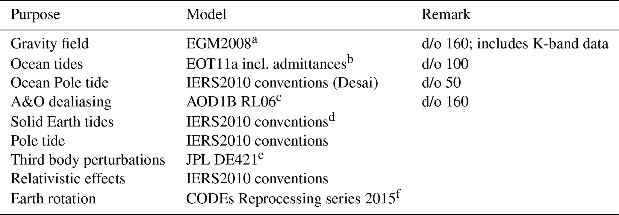
^a Pavlis et al. (2012). ^b Savcenko and Bosch (2011). ^c Dobslaw et al. (2017). ^d Petit and Luzum (2010). ^e Folkner et al. (2009). ^f Sušnik et al. (2016) and Sušnik et al. (2020).

In the second step the a priori orbits are introduced to set up normal equations along the orbit by using the same orbit parametrisation, and additionally, spherical harmonic (SH) coefficients representing the gravity field. The kinematic positions again serve as pseudo-observations and are weighted according to the covariance information. All daily normal equations are accumulated into one normal equation system covering one month, which is eventually solved for in order to obtain a solution for the correction of the orbit parameters and the SH coefficients. No regularisation is applied to compute the gravity field parameters.

To investigate the robustness and the dependencies of the approach, two types of orbit parametrisations were adopted for each type of covariance in orbit reconstruction and gravity field recovery:

• A dynamic orbit represented by only six initial osculating (Keplarian) elements and nine additional parameters characterising the accelerometer, and

• a reduced-dynamic orbit represented by the same parameters as the dynamic orbit and additional constrained Piecewise Constant Accelerations (PCA) set up over intervals of 15 min in radial, along-track and cross-track direction.

The nine additional accelerometer parameters consist of a bias in radial and cross-track direction, a polynomial of degree 3 in along-track and a scaling factor for each axis. The optimal constraining and sampling of the PCAs for the reduced-dynamic orbit are determined empirically. The constraints are set to $\mathrm{1}\times {\mathrm{10}}^{-\mathrm{8}}$ m s⁻², the sampling is set to 15 min.

As the CMA is only one of several approaches to recover gravity field information from kinematic positions, we refer to Baur et al. (2014) for an overview on different strategies of gravity field determination, including a brief description of stochastic modelling.

4 Stochastic noise modelling

The stochastic noise modelling of kinematic orbit positions is a crucial part for high-precision gravity field recovery. The way the noise in the pseudo-observations is treated influences the quality of the result (e.g., in terms of formal errors) significantly, and it might also affect the solution itself. The correct characterisation of noise in the data retains the full signal content and separates signal from noise through a modelling of the latter – provided that the signal component is also adequately modelled.

In case of kinematic positions, which are introduced as pseudo-observations in the CMA, one has to consider the process of calculating these pseudo-observations in the stochastic modelling. The original observations are the GPS dual-frequency carrier phases. The kinematic positions of the LEO satellite are determined at the observation epochs of the GPS carrier phase measurements by a precise point positioning (PPP) approach (Zumberge et al., 1997) where three dimensional coordinates and the receiver clock corrections are estimated. GPS satellite orbits and clocks are introduced as error free, thus, correlations due to the GPS satellite orbits, clocks and underlying network errors are neglected as it is commonly done in most studies. However, the carrier phase ambiguities, which represent the integer number of full cycles between the GPS satellites and the receiver, and additional satellite- and receiver-specific biases, correlate the kinematic positions in time, “implying that degraded estimates of carrier phase ambiguities may affect the estimation of the kinematic positions for more than one hour”. (Jäggi et al., 2011b). Consequently, the positions are no longer uncorrelated and the correlation depends on the constellation of the GPS satellites. Initially, carrier phase ambiguities are estimated as float numbers together with the kinematic coordinates and the receiver clock corrections in the least-squares adjustment. A fixing between satellite differences to the correct integer number, requires in the undifferenced GPS processing the knowledge of satellite-specific bias terms (Schaer et al., 2020). In Sect. 5 an outlook is given on the effect of integer-fixed positions on the stochastic behaviour of the kinematic pseudo-observations.

The kinematic positions are introduced as pseudo-observations in a standard least-squares adjustment to estimate orbit parameters and gravity field parameters in a joint adjustment. The least-squares adjustment yields

$$\begin{array}{}\text{(1)}& \mathit{x}=({\mathbf{A}}^{\mathrm{T}}\mathbf{PA}{)}^{-\mathrm{1}}{\mathbf{A}}^{\mathrm{T}}\mathbf{P}\mathit{l},\end{array}$$

where x is the solution of the linearised system of equations, composed of orbit and gravity field parameters. l denotes the Observed minus Computed (O−C) vector, where the pseudo-observations form the observed vector. A being the first design-matrix and P the weight matrix, which is supposed to describe the stochastic behaviour of the pseudo-observations.

4.1 Formal variance propagation

The process of calculating the pseudo-observations from the original carrier phase measurements allows for a covariance estimation. We derive the covariance matrix ${\mathbf{C}}_{ll}^{\mathrm{formal}}$ from the inverse normal equation matrix, which is the result of a formal variance propagation from the phase observations to the unknown kinematic positions according to

$$\begin{array}{}\text{(2)}& {\mathbf{C}}_{ll}^{\mathrm{formal}}={\mathit{\sigma }}_{\mathrm{0}}^{\mathrm{2}}\left({\mathbf{RQ}}_{kk}{\mathbf{R}}^{\mathrm{T}}\right),\end{array}$$

where

$$\begin{array}{}\text{(3)}& \mathbf{R}:=({\mathbf{A}}^{\mathrm{T}}\mathbf{PA}{)}^{-\mathrm{1}}{\mathbf{A}}^{\mathrm{T}}\mathbf{P}.\end{array}$$

Q_kk denotes the cofactor matrix of the original phase observations and ${\mathit{\sigma }}_{\mathrm{0}}^{\mathrm{2}}$ is the a priori variance of unit weight. The relation between cofactor and covariance matrix can be established by $\mathbf{C}={\mathit{\sigma }}_{\mathrm{0}}^{\mathrm{2}}\mathbf{Q}$. White noise is generally assumed for C_kk. The propagation matrix R stems from the kinematic point positioning with A being the first design-matrix and P the weight matrix derived from ${\mathbf{Q}}_{kk}^{-\mathrm{1}}$.

The correlations in ${\mathbf{C}}_{ll}^{\mathrm{formal}}$ feature a twice-per-revolution signal, which is related to the satellite crossings of the pole and the weaker observation geometry there since GPS satellites revolve in inclined orbits at 55^∘ with respect to the Earth's equator. The better tracking geometry in the equatorial regions leads to a smaller number of interruptions, thus fewer ambiguities, and consequently, to a better determination of each ambiguity and more correlated kinematic positions (Jäggi et al., 2011b). Generally, the correlations are positive and decreasing for a growing distance in time, however jumps may occur due to the set up of new ambiguities, which indicates changes in the observed constellation or data problems, e.g., cycle slips.

The GPS carrier phase ambiguities are the only parameters in A in Eqs. (2) and (3) connecting different epochs when using GPS phase data. Consequently, deficiencies in the modelling of the GPS phase observations may be propagated through the ambiguities over several epochs, which is also reflected by ${\mathbf{C}}_{ll}^{\mathrm{formal}}$. Since ${\mathbf{C}}_{ll}^{\mathrm{formal}}$ only depends on the observation scenario but not on the actual observations (since white noise is assumed for them), any degradation of positions due to GPS data quality issues (including issues with GPS orbits and clocks) is not reflected in this type of covariance information. An outlier in the carrier phase observations, e.g., affects the individual kinematic position and through the ambiguities neighbouring positions as well, but not the formal variance propagation.

The weight matrix P for the least-squares adjustment of the gravity field and orbit parameters (Eq. 1) is determined from the inverse covariance matrix and the a priori variance of unit weight ${\mathit{\sigma }}_{\mathrm{0}}^{\mathrm{2}}$ as

$$\begin{array}{}\text{(4)}& \mathbf{P}={\mathit{\sigma }}_{\mathrm{0}}^{\mathrm{2}}{\mathbf{C}}_{ll}^{-\mathrm{1}}={\mathbf{Q}}_{ll}^{-\mathrm{1}}\end{array}$$

The a priori variance of unit weight ${\mathit{\sigma }}_{\mathrm{0}}^{\mathrm{2}}$ is chosen based on the expectation about the uncertainty of the original carrier phase observations and is usually set between 1 and 2 mm for GPS L1 and L2 data. However, one is free to chose an arbitrary number, limits may only be given by the numerical precision of computers.

Introducing the pseudo-observations together with the full covariance matrix ${\mathbf{C}}_{ll}^{\mathrm{formal}}$ in the least-squares adjustment for the gravity field recovery would be equivalent to starting directly with carrier phase observations (shown for the application of carrier phase observations and kinematic positions as pseudo-observations in Jäggi et al., 2011b). Facing the large number of kinematic pseudo-observations, e.g., 3×8640 for one day with a 10 s sampling of GPS data, this would require a huge computational effort and would demand high storage requirements. Two ways how to deal with these issues are presented in the next sub-sections.

4.1.1 Epoch-wise covariance information

The epoch-wise covariance information is a subset of the covariance matrix from the formal variance propagation, which may be easily derived in the kinematic point positioning process using pre-elimination and back-substitution techniques. Focusing only on the kinematic positions, the epoch-wise covariances, assembled in Eq. (5), consist of six distinct elements, which comprise the variances of the three coordinates ($c_{xx},c_{yy},c_{zz}>\mathrm{0}$) and the off-diagonal elements $c_{xy},c_{xz},c_{yz}$, which contain information about the correlation between the x,y,z axes in the Earth-fixed coordinate system,

$$\begin{array}{}\text{(5)}& {\mathbf{C}}_{\mathrm{epo}}^{\mathrm{formal}}=\left[\begin{array}{ccc}{c}_{xx}& c_{xy}& c_{xz}\\ c_{xy}& c_{yy}& c_{yz}\\ c_{xz}& c_{yz}& c_{zz}\end{array}\right].\end{array}$$

Any correlations between subsequent epochs are neglected. The epoch-wise covariances are only little memory consuming and the 3×3-matrix is invertible to derive the (epoch-wise) weight matrices according to Eq. (4).

The epoch-wise covariance information mainly features the twice-per-revolution behaviour for polar orbiting satellites (orbital period for GRACE was T=96 min) which reflects the observation scenario. Figure 1 displays all elements of the epoch-wise covariance matrix for GRACE-A of day 091, 2007 in the time and frequency domain. The elements are rotated to a Local Orbit Frame (LOF) based on the unit vectors derived from the reduced-dynamic orbit, the axes follow radial (r), along-track (a) and cross-track (c) direction. The twice-per-revolution signal is clearly visible in the radial component at $T/\mathrm{2}=\mathrm{48}$ min where T corresponds to the revolution period of the GRACE satellites.

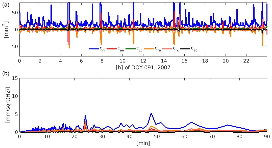
Figure 1 Independent components of the epoch-wise covariance matrix of GRACE-A for one arc, day 091, 2007, in radial (r), along-track (a) and cross-track (c) direction in the time (a) and frequency (b) domain. The amplitude spectrum in the bottom graph shows a clear peak at 48 min corresponding to half of the orbital period.

This information can only be derived from the formal variance propagation and cannot be neglected in the orbit reconstruction and gravity field recovery process without significantly degrading the recovered gravity field solutions using the classical CMA, see Prange (2010).

Impact of epoch-wise covariance information on orbit reconstruction and gravity field recovery

The residuals of the reconstructed orbit (Fig. 2) with respect to the kinematic positions are characterised by the underlying orbit parametrisation. The reduced-dynamic orbit residuals in Fig. 2 (top) show a scatter around zero with few systematics where long-periodic effects related to a deficient force modelling are absorbed by the PCA set up every 15 min. Thus, the reduced-dynamic orbit follows the observations to a large extent. In contrast, the residuals of the dynamic orbit shown in Fig. 2 (middle) feature strong systematic signals caused by the deficient force model, which are mainly visible as once-per-revolution signatures.

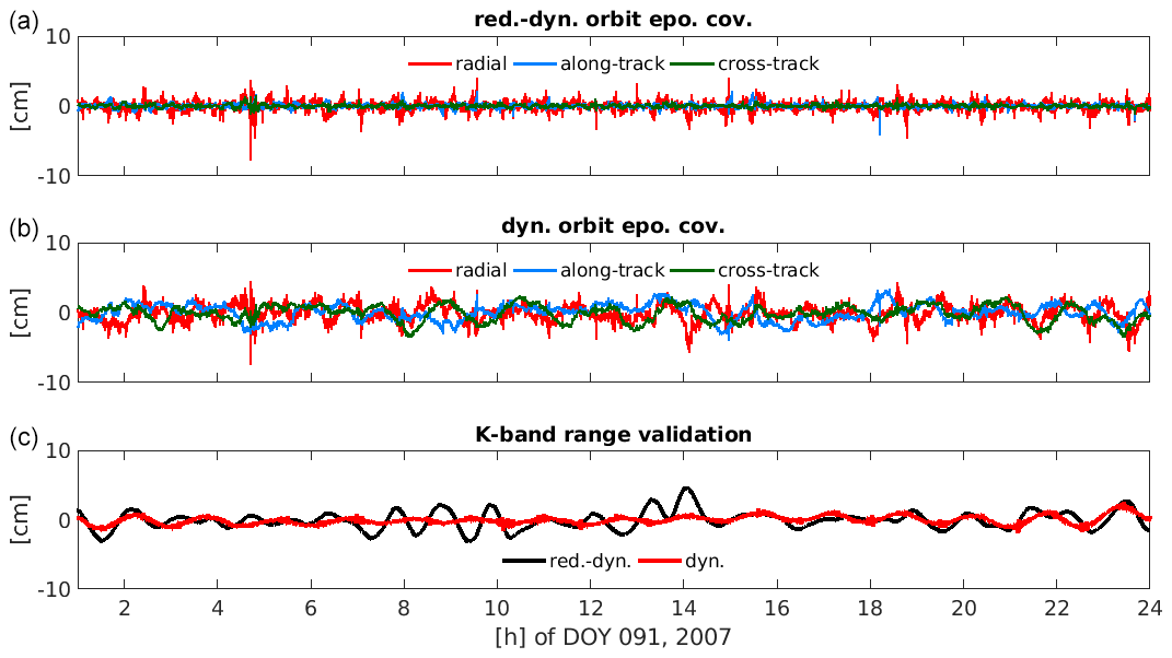
Figure 2 Orbit residuals of GRACE-A using epoch-wise covariances for day 091, 2007, for the reduced-dynamic orbit (a), the dynamic orbit (b), and the respective K-band range validations (c).

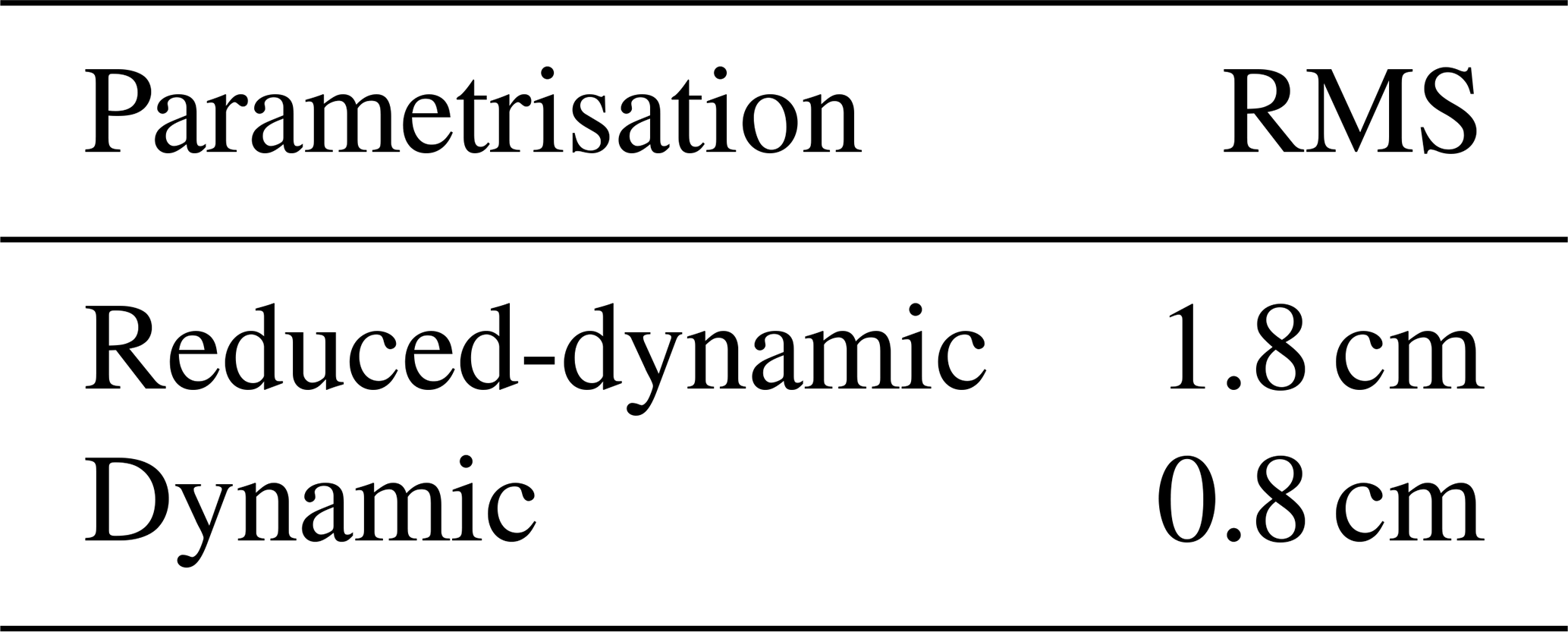
The K-band validation of the fitted dynamic orbit is smoother than of the fitted reduced-dynamic orbit (see Table 2). This reflects that the PCA allow the orbit to follow the excursions in the observations to a certain extent, whereas, the dynamic orbit follows – based on the least-squares adjustment – the a priori force field. The small high-frequency noise in the K-band validation, visible, e.g., in the peaks of the red curve, can be attributed to the high degrees of the gravity field, which are difficult to estimate using only GPS observations. The K-band validation of the reduced-dynamic orbit does not reflect the same level of accuracy as using directly GPS carrier phase observations for orbit determination, which is accounted for by the insufficient stochastic model, see Jäggi et al. (2011b) for a detailed investigation. This means the fitted reduced-dynamic orbit is less precise when being computed from kinematic positions with epoch-wise covariance information than a corresponding orbit being computed directly from GPS carrier phase observations, where no degradation due to neglected correlations is occurring.

Table 2 K-band RMS over all days using epoch-wise covariances in the orbit reconstruction for April 2007.

The gravity field solutions based on the epoch-wise covariance information when using the reduced-dynamic and the dynamic orbit parametrisations are shown in Fig. 3. The solution based on the dynamic orbit parametrisation is degraded because of the deficient force model. The gravity field solution based on the reduced-dynamic parametrisation (red) is of good quality and represents the classical parametrisation used so far in the context of the CMA. In all further degree amplitude figures it will serve as a reference and will always be indicated by red lines. Any further reference such as “classical approach” refers to the use of epoch-wise covariance information.

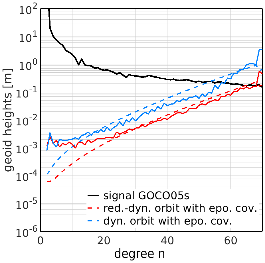
Figure 3 Monthly GRACE GPS-only gravity field solution (April 2007) based on a reduced-dynamic orbit (red) and a dynamic orbit (blue). The solid lines depict the difference degree amplitudes to GOCO05s, the dashed lines denote the formal errors from the least-squares adjustment.

In the dynamic and the reduced-dynamic case the formal errors (dashed lines) of the solution do not reflect the accuracy assessed by the differences to the (superior) GOCO05s (Mayer-Gürr et al., 2015) gravity field model (solid lines). Hence, the stochastic description of the pseudo-observations needs to be expanded.

4.1.2 Covariance information over-arching epochs

Apart from the epoch-wise covariance information from the formal variance propagation, the covariances connecting a certain number of epochs may be taken into account as well. As discussed at the beginning of Sect. 4.1, their behaviour reflects the presence of the carrier phase ambiguities as solely these parameters connect different epochs in a kinematic point positioning. They comprise the observation geometry, thus the influence of the constellation on the correlation between epochs.

The computation of the covariances is in principle straightforward, however, depending on the number of correlated epochs that are of interest, memory consumption may become an issue (e.g., for one day of 10 s kinematic positions and correlations up to two hours >53 Million elements need to be stored, which consumes in a 64 bit notation about 500 MB memory). The variance/covariance matrix is fully populated and nondegenerate if all epochs are considered. However, when taking only correlations for a certain time interval into account, the matrix is band-diagonal and not necessarily invertible anymore. A simple approach of obtaining an invertible matrix is slicing fully populated blocks of the matrix and inverting these blocks individually (the block diagonal matrix is invertible, cf. Jäggi et al., 2011b). The block length defines the number of epochs that are considered. Correlations between individual blocks are neglected, however, when applying a sufficiently long correlation time (until the correlation becomes negligible) the impact on the solution is insignificant. We use the covariance matrix up to 50 min, which is about twice the time the observed constellation takes to vary completely (the maximum time interval an individual ambiguity is valid is around 25 to 30 min, hence, only ambiguities overlapping each other propagate covariance information for longer time spans with decreasing influence the longer the distance in time is). Figure 4 shows all individual elements of the covariance function for the first 50 min of the day 091, 2007 in Earth-fixed frame (panel a) and for a comparison with the subsequent graphs of covariance functions also rotated to a LOF based on a fit using the reduced-dynamic orbit parametrisation (panel b). The largest variance (for c_zz and c_rr) slightly exceeds 50 mm², but for reasons of clarity it is cut off in Fig. 4. However, this number coincides with the fact that the radial component is about three times less precise than the other two axes (visible in Fig. 1).

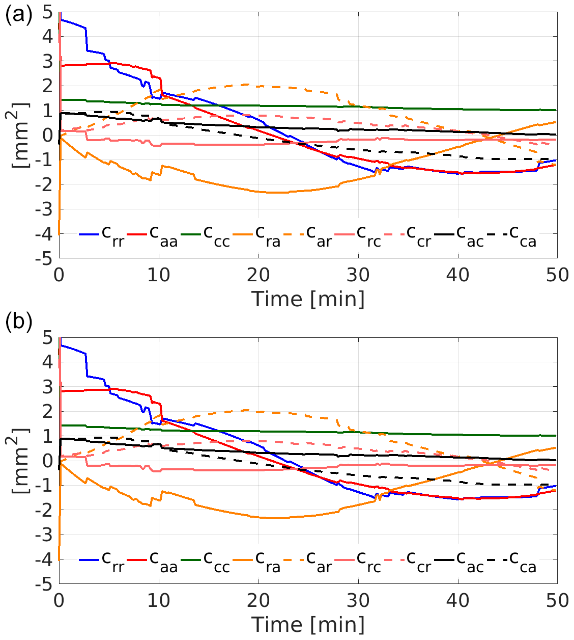
Figure 4 Covariance function over 50 min for kinematic positions of GRACE-A (first 50 min of day 091, 2007) in Earth-fixed reference frame (a) and in LOF (b).

The jumps in the covariance function occur due to the setup of new ambiguities (changes in the observed GPS constellation).

Impact of covariances over 50 min on orbit reconstruction and gravity field recovery

For both, the dynamic and the reduced-dynamic orbit, covariances covering correlations up to 50 min were applied to determine the weight matrix in Eq. (4). The residuals of the reconstructed orbits with respect to the kinematic pseudo-observations in Fig. 5 exhibit a slightly different behaviour compared to the classical approach shown in Fig. 2. The dynamic orbit is still subject to the deficient a priori force model, however long-periodic variations induced by the observation geometry and ambiguity setup of the original phase observations are no longer allowed to be absorbed by orbit parameters. That accounts for both parametrisations and is visible in particular in the reduced-dynamic orbit residuals as superimposed oscillation (see Fig. 5, top).

Figure 5 Orbit residuals of GRACE-A using covariances from the formal variance propagation over a period of 50 min for day 091, 2007, for the reduced-dynamic orbit (a), the dynamic orbit (b) and the respective K-band range validation (c).

The K-band range residuals for the reduced-dynamic orbit are significantly lower than in the classical approach of weighting (cf. Tables 3 and 2) since long-periodic variations of the pseudo-observations are no longer (erroneously) fitted by the parameters of the orbit model but (correctly) interpreted as a consequence of the ambiguity-induced correlations in time (Jäggi et al., 2011b). In contrast to the epoch-wise covariance weighting, the K-band range validation is now at the same level as using directly GPS carrier phase observations for orbit determination. Experiments substantiating this behaviour are presented in Jäggi et al. (2011b).

Table 3 K-band RMS using covariances over 50 min in the orbit reconstruction for April 2007.

Weighting the kinematic positions including 50 min of correlations leads to slightly more realistic formal errors in the gravity field recovery process (Fig. 6). The very low degrees, however, still reveal deficiencies in the stochastic modelling. The dynamic solution profits most from taking the 50 min of correlations into account (compare Fig. 6 to Fig. 3), however, it cannot fully compete with the reduced-dynamic solution in the higher degrees. The very low degrees (best visible for degree 2) are better determined with the dynamic parametrisation as the PCA of the reduced-dynamic parametrisation absorb some of the signal.

Figure 6 GRACE GPS-only gravity field solution for April 2007. Covariances considering correlations over 50 min from the purely formal variance propagation in the determination of the kinematic positions are used to weight the kinematic positions.

4.2 Empirical covariances

The residuals of an orbit fit with respect to the kinematic positions reflect all model (functional and stochastic) and data deficiencies. Consequently, deriving covariances from the residuals leads to a stochastic description of the entire physical system. The residuals e are obtained as the difference between the pseudo-observations l (i.e., the kinematic positions) and the estimated observations, which are computed from the estimated model parameters x with

$$\begin{array}{}\text{(6)}& \mathit{e}=\mathit{l}-\mathbf{A}\mathit{x}.\end{array}$$

As these residuals depend on the a priori force field, we first estimate a gravity field solution based on epoch-wise covariances and then re-introduce this solution as new a priori gravity field, to become independent from the a priori gravity field when computing the residuals for the empirical covariances. This procedure could be applied iteratively by taking the solution computed using empirical covariances as new a priori gravity field, however, in our case of starting with epoch-wise covariances as an initial stochastic model, it turned out that the gravity field solution does not alter after one iteration (not shown). We compute the residuals in a back-substitution process, thus allowing for efficient solving of the normal equations by prior pre-elimination of the orbit parameters.

The covariance function for a certain time interval Δt_k, with k denoting the sampling interval of the pseudo-observations, is defined by the auto-correlation between the respective estimated residuals e according to

$$\begin{array}{}\text{(7)}& \begin{array}{r}{c}_{xx}\left(\mathrm{\Delta }{t}_k\right)={\displaystyle \frac{\mathrm{1}}{n}}\sum _{i=\mathrm{0}}^n{e}_x\left(t_i\right)e_x(t_i+\mathrm{\Delta }{t}_k)\\ c_{yy}\left(\mathrm{\Delta }{t}_k\right)={\displaystyle \frac{\mathrm{1}}{n}}\sum _{i=\mathrm{0}}^n{e}_y\left(t_i\right)e_y(t_i+\mathrm{\Delta }{t}_k)\\ c_{zz}\left(\mathrm{\Delta }{t}_k\right)={\displaystyle \frac{\mathrm{1}}{n}}\sum _{i=\mathrm{0}}^n{e}_z\left(t_i\right)e_z(t_i+\mathrm{\Delta }{t}_k)\end{array}.\end{array}$$

This type of auto-correlation is only legitimate under the assumption that the residuals in the considered interval fulfil the requirements of a (weak) stationary process (Etten, 2005). We assume the noise to be stationary, thus, the more parameters are set up to absorb deficiencies in the modelling, the better this assumption is fulfilled, which can be seen in the orbit residuals of the dynamic and reduced-dynamic parametrisation. Moreover, the longer the correlation lengths are that are taken into account, the more coloured is the noise in the residuals (to be clearly seen in Figs. 2 and 5 for the reduced-dynamic cases).

The correlations between the axes are obtained through a cross-correlation between the residuals of the respective axes

$$\begin{array}{}\text{(8)}& \begin{array}{r}{c}_{xy}\left(\mathrm{\Delta }{t}_k\right)={\displaystyle \frac{\mathrm{1}}{n}}\sum _{i=\mathrm{0}}^n{e}_x\left(t_i\right)e_y(t_i+\mathrm{\Delta }{t}_k)\\ c_{xz}\left(\mathrm{\Delta }{t}_k\right)={\displaystyle \frac{\mathrm{1}}{n}}\sum _{i=\mathrm{0}}^n{e}_x\left(t_i\right)e_z(t_i+\mathrm{\Delta }{t}_k)\\ c_{yx}\left(\mathrm{\Delta }{t}_k\right)={\displaystyle \frac{\mathrm{1}}{n}}\sum _{i=\mathrm{0}}^n{e}_y\left(t_i\right)e_x(t_i+\mathrm{\Delta }{t}_k)\\ c_{yz}\left(\mathrm{\Delta }{t}_k\right)={\displaystyle \frac{\mathrm{1}}{n}}\sum _{i=\mathrm{0}}^n{e}_y\left(t_i\right)e_z(t_i+\mathrm{\Delta }{t}_k)\\ c_{zx}\left(\mathrm{\Delta }{t}_k\right)={\displaystyle \frac{\mathrm{1}}{n}}\sum _{i=\mathrm{0}}^n{e}_z\left(t_i\right)e_x(t_i+\mathrm{\Delta }{t}_k)\\ c_{zy}\left(\mathrm{\Delta }{t}_k\right)={\displaystyle \frac{\mathrm{1}}{n}}\sum _{i=\mathrm{0}}^n{e}_z\left(t_i\right)e_y(t_i+\mathrm{\Delta }{t}_k)\end{array}.\end{array}$$

Assembling a variance/covariance matrix from the covariance function leads to a block Toeplitz structure, which may be populated by

$$\begin{array}{}\text{(9)}& \mathbf{cov}\left(\mathrm{\Delta }{t}_k\right)=\left[\begin{array}{cccc}{c}_{xx}\left(\mathrm{\Delta }{t}_k\right)& c_{xy}\left(\mathrm{\Delta }{t}_k\right)& c_{xz}\left(\mathrm{\Delta }{t}_k\right)& \\ c_{yx}\left(\mathrm{\Delta }{t}_k\right)& c_{yy}\left(\mathrm{\Delta }{t}_k\right)& c_{yz}\left(\mathrm{\Delta }{t}_k\right)& \\ c_{zx}\left(\mathrm{\Delta }{t}_k\right)& c_{zy}\left(\mathrm{\Delta }{t}_k\right)& c_{zz}\left(\mathrm{\Delta }{t}_k\right)\end{array}\right]\end{array}$$

and

$$\begin{array}{}\text{(10)}& {\mathbf{C}}_{ee}=\left[\begin{array}{ccc}\mathbf{cov}\left(\mathrm{\Delta }{t}_{\mathrm{0}}\right)& \mathbf{cov}\left(\mathrm{\Delta }{t}_{\mathrm{1}}\right)& \mathbf{cov}\left(\mathrm{\Delta }{t}_{\mathrm{2}}\right)\\ {\mathbf{cov}}^{\mathrm{T}}\left(\mathrm{\Delta }{t}_{\mathrm{1}}\right)& \mathbf{cov}\left(\mathrm{\Delta }{t}_{\mathrm{0}}\right)& \mathbf{cov}\left(\mathrm{\Delta }{t}_{\mathrm{1}}\right)\\ {\mathbf{cov}}^{\mathrm{T}}\left(\mathrm{\Delta }{t}_{\mathrm{2}}\right)& {\mathbf{cov}}^{\mathrm{T}}\left(\mathrm{\Delta }{t}_{\mathrm{1}}\right)& \mathbf{cov}\left(\mathrm{\Delta }{t}_{\mathrm{0}}\right)\\ \mathrm{\ddots }& \mathrm{\ddots }& \mathrm{\ddots }\end{array}\right].\end{array}$$

In case of correlating less than all epochs, the matrix is band diagonal. Note that only for Δt₀ the relation for the off-diagonal elements of c_xy=c_yx, c_xz=c_zx, c_yz=c_zy holds, in case of $\mathrm{\Delta }{t}_k,k\ge \mathrm{1}$ the covariance block cov(Δt_k) is composed of nine independent elements.

We do not want to model short term variations within an arc, therefore, we use the residuals of a whole month to derive a mean covariance function. The use of empirical covariances relies on the quality and the shape of the residuals, in particular outliers will affect the empirical covariances heavily. This leads to an interdependency between the orbit parametrisation and the pseudo-observations. The dependency on the a priori gravity field is mitigated as much as possible by first estimating an independent gravity field solution and obtaining the covariance function from post-fit residuals. Consequently, the time until the correlations become negligible is highly dependent on these two factors. Even under the assumption that there are no outliers (a prerequisite) in the data, the parametrisation of the underlying orbit affects the magnitude and time the correlations take to vanish significantly, see Fig. 7 for the two parametrisations adopted in this study.

We introduce the epoch-wise covariance information from the formal variance propagation into the a priori gravity field and orbit recovery, on which the empirical covariance function is built, because the epoch-wise covariances transport information about the tracking scenario (inferior constellation over polar regions), which cannot be easily recovered by orbit dynamics only. However, introducing white noise as most simple assumption to weight the kinematic positions in the a priori gravity field and orbit recovery, leads to the same gravity field solution, but requires at least one additional iteration.

Memory consumption is not an issue for the usage of empirical covariances since they are valid over one month and are fully described by one function from which the variance-/covariance matrix can be compiled according to Eq. (10).

We expect the nature of the residuals in a LOF to be more stationary, as periodic behaviours due to the satellites' orbit will be reflected much cleaner and easier to interpret, thus, we derive the empirical covariances in a LOF. For the reduced-dynamic orbit the largest correlations over epochs occur in the radial direction, which can be attributed to the simultaneous estimation of kinematic positions and receiver clock corrections, while the other directions play a minor role. This is different for the dynamic parametrisation, where the correlations in all three axes are about the same magnitude. Noteworthy is the large and long lasting correlation in cross-track and between the radial and the along-track axis. Thus, the three axis are not independent from each other, even over several epochs.

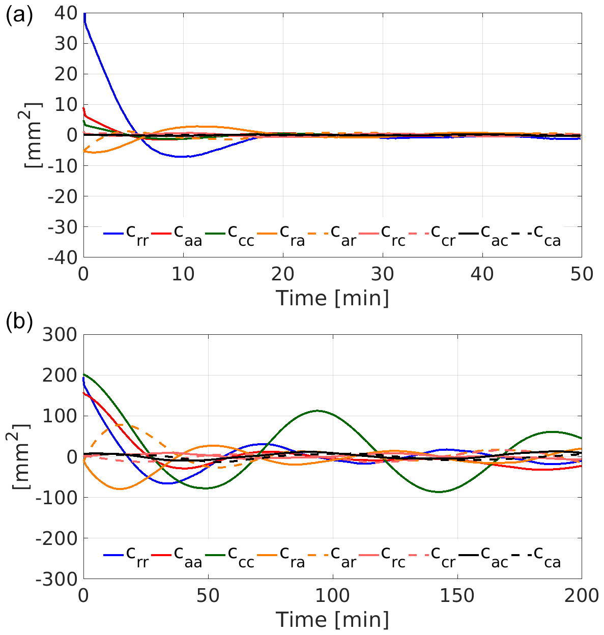
Figure 7 Empirical covariance function derived from the reduced-dynamic orbit residuals (a) and dynamic orbit residuals (b) of GRACE-A over one month for a period of 50 and 200 min and in a LOF composed of radial (r), along-track (a) and cross-track (c).

As we aim to reconstruct the weighting for the observations from estimated residuals e, the relation between the covariance matrix of the residuals C_ee and the covariance matrix of the observations is needed. This relation may be established by variance propagation starting from inserting Eq. (1) into Eq. (6)

$$\begin{array}{}\text{(11)}& \begin{array}{rl}\mathit{e}& =\mathit{l}-\mathbf{A}\mathit{x}\\ & =\mathit{l}-\mathbf{A}\left[({\mathbf{A}}^{\mathrm{T}}\mathbf{PA}{)}^{-\mathrm{1}}{\mathbf{A}}^{\mathrm{T}}\mathbf{P}\mathit{l}\right]\\ & =\left[\mathbf{I}-\mathbf{A}({\mathbf{A}}^{\mathrm{T}}\mathbf{PA}{)}^{-\mathrm{1}}{\mathbf{A}}^{\mathrm{T}}\mathbf{P}\right]\mathit{l}.\end{array}\end{array}$$

Setting

$$\begin{array}{}\text{(12)}& \mathbf{S}:=\left[\mathbf{I}-\mathbf{A}({\mathbf{A}}^{\mathrm{T}}\mathbf{PA}{)}^{-\mathrm{1}}{\mathbf{A}}^{\mathrm{T}}\mathbf{P}\right],\end{array}$$

the variance propagation for the covariance matrix of the estimated residuals follows

$$\begin{array}{}\text{(13)}& {\mathbf{C}}_{ee}={\mathit{\sigma }}_{\mathrm{0}}^{\mathrm{2}}\left({\mathbf{SQ}}_{ll}{\mathbf{S}}^{\mathrm{T}}\right),\end{array}$$

which gives by expansion of the products

$$\begin{array}{}\text{(14)}& {\mathbf{C}}_{ee}={\mathbf{C}}_{ll}-{\mathit{\sigma }}_{\mathrm{0}}^{\mathrm{2}}\left[\mathbf{A}({\mathbf{A}}^{\mathrm{T}}\mathbf{PA}{)}^{-\mathrm{1}}{\mathbf{A}}^{\mathrm{T}}\right].\end{array}$$

A simple re-arrangement yields

$$\begin{array}{}\text{(15)}& {\mathbf{C}}_{ll}={\mathbf{C}}_{ee}+{\mathit{\sigma }}_{\mathrm{0}}^{\mathrm{2}}\left[\mathbf{A}({\mathbf{A}}^{\mathrm{T}}\mathbf{PA}{)}^{-\mathrm{1}}{\mathbf{A}}^{\mathrm{T}}\right],\end{array}$$

when deploying the residuals e as estimation for the covariance matrix of the observations C_ll. For the processing of kinematic positions with a precision of about 1 cm, the correctional term ${\mathbf{C}}_{\widehat{l}\widehat{l}}={\mathit{\sigma }}_{\mathrm{0}}^{\mathrm{2}}\left[\mathbf{A}({\mathbf{A}}^{\mathrm{T}}\mathbf{PA}{)}^{-\mathrm{1}}{\mathbf{A}}^{\mathrm{T}}\right]$ will be negligible with respect to C_ee and we may set

$$\begin{array}{}\text{(16)}& {\mathbf{C}}_{ll}\approx {\mathbf{C}}_{ee},\end{array}$$

even though the estimation of the covariance matrix of the observations is then not unbiased anymore. Figure 8 shows the correctional term ${\mathbf{C}}_{\widehat{l}\widehat{l}}$ for the first minutes of day 091, 2007 for the reduced-dynamic (panel a) and dynamic (panel b) orbit parametrisation. The correctional term is given in a LOF and can be directly compared to the empirical covariance functions in Fig. 7. The first minutes of the arc feature the largest correctional term, which is located at the arc's boundaries, a consequence of the least-squares adjustment. It gets smaller towards to the middle of the arc.

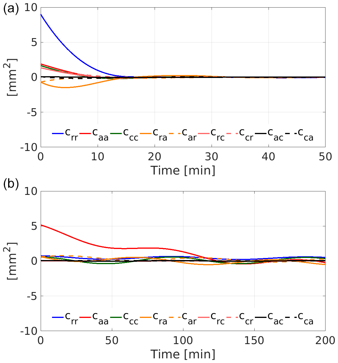
Figure 8 First minutes of the correctional term for the reduced-dynamic orbit parametrisation (a) and the dynamic orbit parametrisation (b) of day 091, 2007, in LOF.

Figure 9 Orbit residuals for day 091, 2007, of GRACE-A using empirical covariances derived for a correlation length of 50 min averaged over April 2007 for the reduced-dynamic orbit (a), the dynamic orbit (b) and the respective K-band range validation (c).

The magnitude of the corrections is much lower than that of the covariance function computed from the residuals (compare graphs in Figs. 7 and 8). The differences in magnitude may be explained by the different nature of C_ee and ${\mathbf{C}}_{\widehat{l}\widehat{l}}$. The correctional term is composed of a purely mathematical variance propagation, thus only reflecting formal errors, which uniquely depend on the feasibility of estimating the orbit parameters for the given observation scenario. In case of the dynamic orbit, the 15 parameters which are set up, are well determined with a low RMS and high redundancy, despite the fact that the overall fit exhibits deficiencies (see residuals in Fig. 2). In case of adding PCA to form the reduced-dynamic parametrisation, the fit is significantly improved but the redundancy is slightly worse and so is the precision of each parameter, however, in both cases the variance propagation of the parameters' precision to estimated observations, reflects this high degree of redundancy.

The covariance function of the residuals on the other hand reflects all model and data deficiencies, and consequently, its magnitude is significantly larger. Neglecting the correctional term provides the benefit of obtaining a nondegenerate covariance matrix by the auto- and cross-correlations. This simplification might only be allowed for kinematic positions, but not for significantly more precise observables such as ultra-precise K-Band observations.

The weight matrix is obtained through Eq. (4). Likewise to the formally propagated covariances, the band diagonal structure is broken up for the sake of simple computation to a block-wise treatment in the least-squares problem (since a band diagonal version of a positive definite matrix is not necessarily positive definite), where one block is invertible and the blocks are independent from each other. The block length depends on the time interval of the auto-correlation of the residuals. The longer, the more computational effort needs to be carried out for the inversion. If the correlation is as such that only one block remains (e.g., one day for a daily arc), C_ll is fully populated and nondegenerate. The block-wise treatment disregards correlations between subsequent blocks including the large correlations between the old block's end and the new block's beginning. Correlations between subsequent blocks do not vanish, however, correlations within a block tend to zero.

Impact of empirical covariances on orbit reconstruction and gravity field recovery

For both orbit parametrisations a weight matrix derived from empirical covariances covering correlations up to 50 min was introduced in the least-squares adjustment. The empirical covariances for the dynamic orbit were determined utilising the dynamic orbit parametrisation, the empirical covariances for the reduced-dynamic orbit from a reduced-dynamic a priori orbit fit. Even though the correlations in the dynamic case do not vanish after 50 min, this time interval is sufficiently long to describe the noise behaviour. The orbit residuals of the fit with empirical covariances and the K-band validation (Fig. 9) show almost the same behaviour as in the classical approach (Fig. 2), an indication that the empirical covariances do not introduce systematic behaviour into the physical system. The K-band RMS over one month is 1.8 cm for the reduced-dynamic and 0.8 cm for the dynamic parametrisation.

Using the empirical covariances to weight the kinematic positions in the gravity field recovery process, one can find formal errors much closer to the degree variance differences (Fig. 10). The low to medium degree terms, which are prone to systematic errors (e.g., antenna phase centre variations, cf. Jäggi et al., 2009b), still feature discrepancies between the theoretically expected errors and the differences to the superior solution.

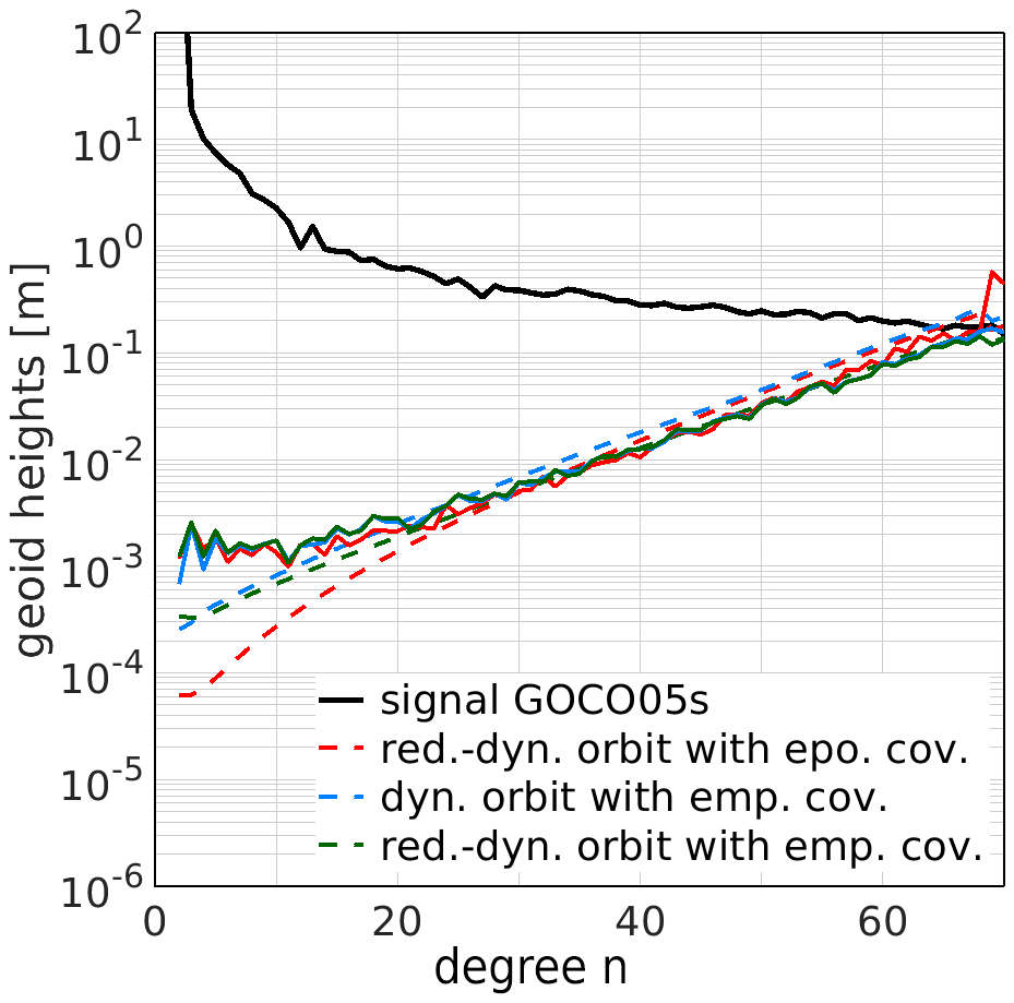
Figure 10 GRACE GPS-only gravity field solution for April 2007. Empirical covariances based on the observation residuals are introduced in the gravity field determination process. These covariances are determined as a mean function over one month and include correlations over 50 min.

Empirical covariances perform better than formally propagated ones because knowledge about model and data deficiencies is both transferred into the least-squares adjustment. Degrees 10 to 26 are slightly degraded compared to the classical solution (Fig. 10, red curve), which needs further inspection. The influence of the PCA is still visible in the low degrees, however, the dynamic solution is not degraded in the higher degrees anymore (compare with Fig. 3) because the empirical covariances are capable of dealing with noise that is absorbed by the PCA.

5 Undifferenced ambiguity fixed positions

In this section we give a short outlook on the use of undifferenced ambiguity fixed kinematic positions for gravity field determination. The process of undifferenced ambiguity fixing can be found in Schaer et al. (2020).

Introducing such kinematic positions potentially helps to improve the gravity field determination process as indicated by the performance of the K-band validation of a classical reduced-dynamic orbit (see Fig. 11). The long-periodic noise gets drastically reduced and the fit of the kinematic positions agrees much better with the K-band range observations (RMS over one month: 0.24 cm compared to 1.8 cm). It is lower as if one employs the formally propagated covariance matrix over a sufficient amount of epochs and close to a double-difference ambiguity fixed baseline solution where sub-millimetre K-Band validations can be achieved (Jäggi et al., 2009a).

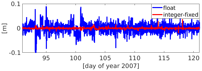
Figure 11 K-band range validation for one month of reduced-dynamic orbit fits of GRACE kinematic positions using epoch-wise covariances.

In the processing of carrier phase observations as many ambiguities as possible are resolved to their integer values before the least-squares adjustment for the kinematic positions takes place, and only the unresolved ambiguities remain in the system. Thus, the number of ambiguity parameters is significantly reduced by more than 90 %. This implies that the kinematic positions are almost uncorrelated in time, which is shown in Fig. 12. Note the differences to the covariance from the corresponding ambiguity float solution in Fig. 4. The correlations vanish after less than ten minutes in the ambiguity-fixed case.

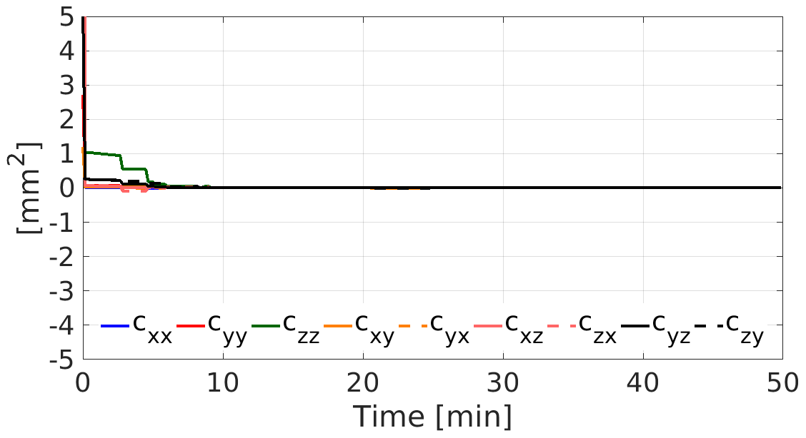
Figure 12 Covariance function over 50 min for undifferenced ambiguity fixed kinematic positions (first 50 min of day 091, 2007 expressed in Earth-fixed reference frame).

In theory, these short correlations in time carry the whole information on the stochastic behaviour. However, for a gravity field solution it is not sufficient to introduce only these correlations in the least-squares adjustment to obtain a reasonably realistic description of the stochastic behaviour; the system behaves almost like employing epoch-wise covariances, which could be expected from the shape of the covariance function and the K-band validation results. The formal errors of the gravity field solution are at the same level as Fig. 3 shows for float solutions. Thus, the correlations over-arching epochs up to 30 min and more, which cannot be reflected in the covariance matrix of the integer-fixed positions anymore, transport essential information about the noise characteristics. In other words, the ambiguity fixing process does not obliterate the correlations (it diminishes them slightly) but it narrows the possibilities of mapping them.

Using undifferenced ambiguity fixed positions together with empirical covariances yields results at the same level as float ambiguities and empirical covariances (not shown). Concerning the signal content in the kinematic positions for gravity field recovery, currently the use of ambiguity fixed positions does not outperform results from a float solution.

6 Conclusions

Kinematic positions are widely used pseudo-observations in gravity field determination and their stochastic behaviour plays a crucial role when assessing the quality of gravity field solutions. Kinematic positions are correlated in time due to the ambiguities in the original GPS phase observations and not considering these correlations degrades a subsequent gravity field solution. Taking these correlations into account can be achieved either by the covariance information of the kinematic positions over longer time spans or by empirical covariances derived from residuals of an orbit fit with respect to the kinematic positions. However, these empirical covariances demand a stationary process and are, therefore, highly dependent on the quality and shape of the residuals.

Formally propagated covariances over-arching epochs are in case of a dynamic orbit parametrisation able to absorb parts of the errors caused by a deficient force field, piecewise constant accelerations have similar capabilities for reduced-dynamic parametrisations. Empirical covariances support the estimation of physically meaningful formal errors and absorb errors caused by a deficient force field in case of dynamic and reduced-dynamic orbit descriptions.

Undifferenced ambiguity fixed kinematic positions feature different stochastic characteristics than ambiguity float kinematic positions – they are almost uncorrelated – however, the possibility of describing the deficiencies that are still in the processing chain is lost through the ambiguity fixing process. Currently, an improvement of a gravity field solutions by using ambiguity-fixed kinematic positions as pseudo-observations cannot be substantiated.

Further steps to investigate the described methods of stochastic modelling include the diversification to different satellite missions, such as Swarm or GOCE, and an appropriate treatment of deteriorated data (affected by outliers etc.), for empirical covariances.