The effect of a density gradient in groundwater on ATES system efficiency and subsurface space use

A heat pump combined with Aquifer Thermal Energy Storage (ATES) has high potential in efficiently and sustainably providing thermal energy for space heating and cooling. This makes the subsurface, including its groundwater, of crucial importance for primary energy savings. ATES systems are often placed in aquifers in which salinity increases with depth. This is the case in coastal areas where also the demand for ATES application is high due to high degrees of urbanization in those areas. The seasonally alternating extraction and re-injection between ATES wells disturbs the preexisting ambient salinity gradient causing horizontal density gradients, which trigger buoyancy flow, which in turn affects the recovery efficiency of the stored thermal energy.

This section uses analytical and numerical methods to understand and explain the impact of buoyancy flow on the efficiency of ATES in such situations, and to quantify the magnitude of this impact relative to other thermal energy losses. The results of this research show that losses due to buoyancy flow may become considerable at (a relatively large) ambient density gradients of over 0.5 kg m⁻³ m⁻¹ in combination with a vertical hydraulic conductivity of more than 5 m day⁻¹. Monowell systems suffer more from buoyancy losses than do doublet systems under similar conditions.

1 Introduction

1.1 Motivation and goal

The application of seasonal Aquifer Thermal Energy Storage (ATES) contributes to meet goals for energy savings and greenhouse gas (GHG) emission reductions. The basic principle of ATES is its use of the subsurface to overcome the seasonal discrepancy between the availability and demand for thermal energy in the built environment. Buildings in moderate climates generally have a heat surplus in summer and a heat shortage in winter. Where groundwater is present in sandy layers (aquifers) of sufficient thickness and hydraulic conductivity, thermal energy can be stored in and extracted from the subsurface. An ATES system consists of one or more pairs of tube wells that infiltrate and simultaneously extract groundwater to store and extract heat. They do so by changing the groundwater temperature by means of a heat exchanger that is connected to the associated building (Fig. 1).

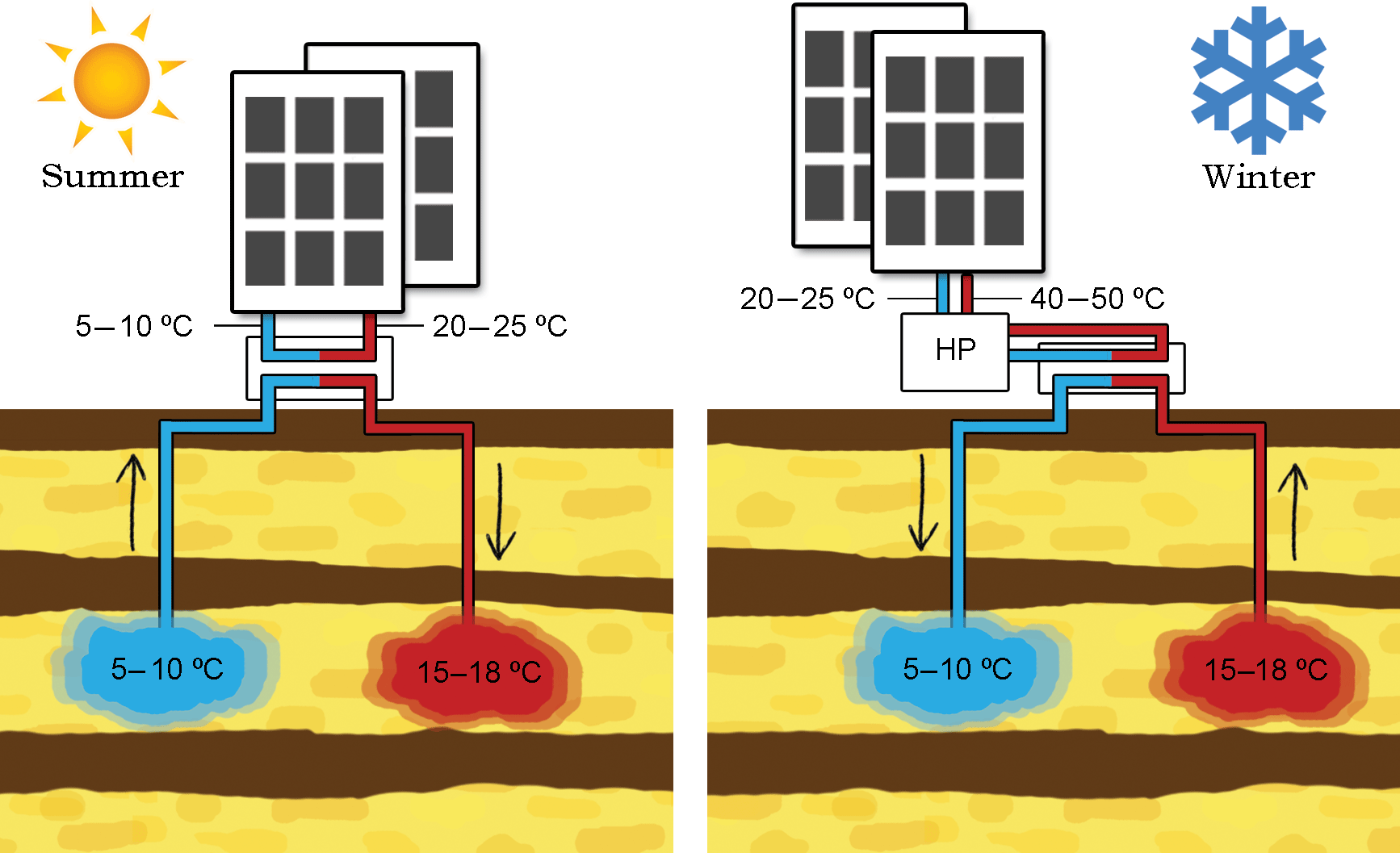
Figure 1 Working principle of an Aquifer Thermal Energy Storage system. In The Netherlands Aquifer thickness ranges from 10 to 160 m.

ATES systems concentrate in urban areas, because their wells have to be placed in close vicinity to their associated building to limit connection costs and heat losses during transport. The world's largest urban areas continue to expand near seas and oceans, making them future hot spots for ATES systems (Bloemendal et al., 2015). Yet, groundwater in coastal areas is often brackish to saline with increasing salinity and, therefore, increasing density with depth (Caljé, 2010; Massmann et al., 2006; Ward et al., 2007). Because ATES wells penetrate aquifers over substantial depths (50–200 m under Dutch conditions), groundwater with different salt concentrations enters the well screens and is subsequently mixed inside these wells and the piping circuit. After heat exchange with the associated building, the groundwater is injected into the same aquifer with a uniform but possibly time-varying salt concentration. This re-injection disturbs the preexisting ambient density distribution. It also causes horizontal density gradients, which trigger buoyancy flow. This buoyancy flow influences the spatial distribution of the injected water and heat and, therefore, also has an impact on the recovery efficiency of the thermal energy stored in the subsurface. The influence of an initially vertical ambient density gradient on the immediate and long-term recovery efficiency of ATES systems has not yet been studied in detail. As a consequence, it has hitherto not been taken into account in the design and operation of ATES systems. Only Caljé (2010) identified the problem and used numerical simulations to analyze the density impact for one specific ATES system in Amsterdam. The current study aims to systematically evaluate how disturbance of the pre-existing salinity distribution in the aquifer that is caused by ATES operations affects their thermal efficiency and their use of subsurface space. This analysis requires identification of which parameters affect the buoyancy most; these parameters can then also be used to identify possible controls to limit the associated heat losses.

1.2 Buoyancy flow around ATES wells

Warm and cold ATES well screens can either be separated horizontally, in which case each pair is called a doublet, or vertically in a single borehole, in which case the screen pair is called a monowell (Fig. 2). The buoyancy flow behaves differently at doublets compared to monowells. The two systems are, therefore, discussed separately. The behavior of the buoyancy flow is schematically shown in Fig. 3 for both types of ATES wells, where Fig. 3a illustrates a doublet and Fig. 3b a monowell.

Figure 2 Schematic representation of ATES doublet and monowell.

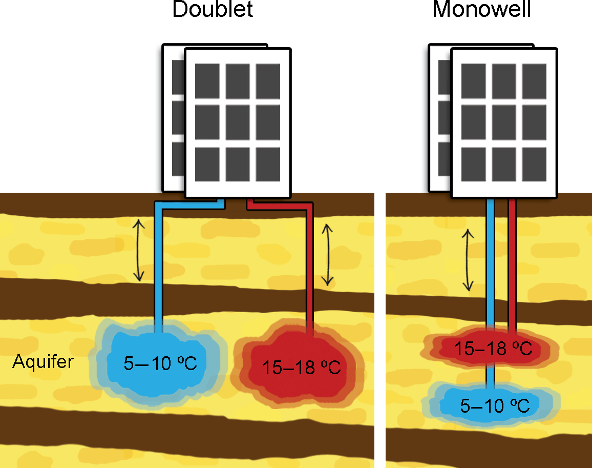
Figure 3 Schematic representation of disturbance of a density gradient by warm well of a doublet (a) and monowell (b) ATES system. At the doublet system the well screen is fully penetrating the aquifer. At the monowell, the warm well is at the top, and cold well at the bottom 1∕3rd of the aquifer.

1.2.1 Doublets

The yellow gradient color in Fig. 3a, indicates that the ambient groundwater density becomes larger with depth. The first storage period is summer, warm water is injected in the warm well (cold well is not depicted). The injected water has a uniform density as is indicated by the uniform yellow, which is the result of mixing of the water, pumped from the paired well of the doublet. The injected water is, therefore, lighter than the groundwater near the bottom of the aquifer and heavier than the groundwater near the top of the aquifer. Hence, the interface tilts towards the well, both at the top and the bottom of the aquifer. This mechanism causes the interface between injected and ambient water to remain vertical in the middle of the aquifer, where the density of the injected water practically equals that of the ambient groundwater at that depth. The injected heat will cause a sharp temperature interface with the ambient groundwater due to thermal retardation (Bloemendal and Hartog, 2018; Doughty et al., 1982) and the fact the spreading of heat is conduction dominated (Bloemendal and Hartog, 2018). The injected water will eventually end up in the middle of the aquifer where ambient and infiltrated densities match. However, after the seasonal storage period, the infiltrated water is extracted again (Fig. 3, A3), at least to the extent possible.

The red color marks where the groundwater and aquifer temperature is changed by the injection. Note that the temperature interface lags behind that of the density interface, due to thermal retardation (e.g. Bloemendal and Hartog, 2018). The thermal retardation adds complexity; it separates the temperature and salinity interfaces. Both interfaces are illustrated in Fig. 3a. The buoyancy-induced flow is strongest at the density interface, and does not fully exercise its tilting effect at the temperature interface. Nevertheless, the buoyancy flow during infiltration, storage and recovery has as a consequence that not all the previously stored water and heat can be extracted later; some is left behind and at least some water with ambient density and temperature is extracted instead, which affects the temperature of the extracted water.

1.2.2 Monowell

Due to the well screens at the top and bottom of the aquifer, the density differences between the ambient and infiltrated water are larger than in the case of a doublet. This results in stronger buoyancy flow. The water extracted from the lower screen has a higher density than the ambient groundwater opposite the upper screen through which it is re-injected. Therefore, the interface between injected and ambient groundwater tilts inward near the top of the screen and outward near the bottom. This water also sinks because of its higher density with respect to the ambient water between the upper and lower screens, Fig. 3 (B1 and B2). The interface tilts faster near the top of the upper screen than near its bottom where the density difference between injected and ambient groundwater is less. The opposite happens when the mixed water from the top screen is injected through the bottom screen, where it encounters heavier ambient groundwater. The interface will tilts faster towards the well near the bottom of the screen than near its top where the density difference between the injected and ambient groundwater is less. At the same time the injected bubble tends to float upwards. The tilting causes early entry of native groundwater into the extracting screens. This is associated with a loss of thermal energy and, therefore, with a loss of thermal efficiency of the ATES system involved. At the same time, such mixing dilutes the interface into a transition zone, which will also reduce the tilting velocity over time, and with a growing number of seasonal cycles. In the longer run, the buoyancy flow and its associate energy losses may, therefore, become negligible.

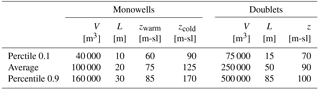
Table 1 ATES-well properties in Amsterdam (rounded) (of Noord-Holland, 2016), V = seasonal storage volume, L = screen length, z = depth of top of screen.

1.3 Approach

This paper is divided into three parts to identify the main drivers, parameters and possible controls of buoyancy flow around ATES wells.

• The specific working conditions are identified first. Both ATES systems and geohydrological characteristics are considered, which define the scenarios to be analyzed. Next to defining an assessment and simulation framework, this first part provides the parameter values necessary to identify the strength and effect of buoyancy flow around ATES wells.

• The second part applies analytical tools to determine the magnitude of the buoyancy flow and its expected effect on the thermal efficiency of the wells. This part serves to provide insight into which parameters affect buoyancy flow most, and when buoyancy may be neglected.

• Numerical simulation is used to deal with the complex behavior of the combined processes of buoyancy, heat conduction, hydro-dynamical dispersion, mixing, repetitive storage and injection, and retardation of the thermal front.

2 Method and materials

2.1 Working conditions and scenarios

2.1.1 ATES systems characteristics

ATES systems in The Netherlands cover a wide range of subsurface thermal energy storage capacity, which mainly depends on the size of the associated building. In sufficiently thick aquifers, like the 150 m thick one below the city of Amsterdam, around 40 % of the ATES systems are monowells, see summary in Table 1. The storage volumes of these systems correspond with those presented in Bloemendal and Hartog (2018). However, due to the large thickness of the aquifer and the larger buildings served, ATES systems in Amsterdam tend to be larger and to have longer screens than those elsewhere in the Netherlands, where aquifers are thinner and cities are smaller.

2.1.2 Geohydrological conditions

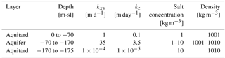
In the Netherlands, ATES is applied in aquifers with a thickness between 10 and 150 m (Bloemendal and Hartog, 2018). This wide range overlaps with that in most other countries, which allows generalizing the Dutch experience. The horizontal hydraulic conductivity in those aquifers ranges from 5 to 50 m day⁻¹ (Bloemendal and Hartog, 2018), vertical anisotropy ratio between 2 and 20 (Xynogalou, 2015) (derived from well test data in Dutch aquifers), which results in a vertical hydraulic conductivity range from 0.25 to 25 m day⁻¹. The salinity gradient strongly depends on local geohydrologic conditions and the material and geologic history of the aquifer. Aquifers near the coast to the extent that they have sufficient continuous recharge, have a relatively sharp interface between fresh and saline water. Aquifers with zero or little recharge tend to have a smooth, up to an almost constant vertical density gradient (Robinson et al., 2006; Stuyfzand, 1993).

Table 2 geohydrological conditions in Amsterdam (Caljé, 2010).

2.1.3 Scenarios

To obtain insight under what circumstances a vertical density gradient in the aquifer may have a considerable impact on thermal energy performance of ATES systems, the analysis in this study uses the conditions identified in Tables 1 and 2:

• Storage volumes per well are between 40 000 and 500 000 m³ yr⁻¹. The storage and recovery is distributed over a year following a block or sine function to represent the seasonal operation scheme.

• The infiltration temperature is 5 and 15 ^∘C for the cold and warm well respectively.

• Well-screen lengths and aquifer thickness are between 10 and 150 m.

• The vertical density gradient is linear and varies from 0.05 to 1 kg m⁻³ m⁻¹. The smallest gradient represents a thick aquifer with fresh water at the top and brackish water at the bottom; the largest gradient represents the extreme case of a thin aquifer of about 35 m thickness with fresh groundwater at the top and seawater at the bottom. A typical value for the density gradient in Dutch aquifers varies between 0.1 and 0.25 kg m⁻³ m⁻¹ (e.g. Caljé, 2010).

• The vertical hydraulic conductivities studied are low (0.5 and 1 m day⁻¹), medium (5 and 10 m day⁻¹) and high (25 m day⁻¹) respectively.

• Losses due to interactions between wells are not taken into account in this section; wells are assumed to be placed at sufficiently large distance from each other, i.e. on at least 3 times the thermal radius (Sect. 2.2) for doublets (NVOE, 2006) and on 1∕3rd of the aquifer thickness for monowells (Xynogalou, 2015).

2.2 Assessment framework

2.2.1 Thermal recovery efficiency

The thermal energy stored in an ATES system can have a positive and negative temperature difference between the infiltrated water and the surrounding ambient groundwater, for either heating or cooling purposes (Fig. 1). In this study the thermal energy stored is referred to as heat or thermal energy; however, all the results discussed equally apply to storage of cold water used for cooling. As in other ATES studies (Doughty et al., 1982; Sommer et al., 2015), the recovery efficiency (η_th) of an ATES well is defined as the amount of injected thermal energy that is recovered after the injected volume has been extracted. For this ratio between extracted and infiltrated thermal energy (E_out∕E_in), the total infiltrated and extracted thermal energy is calculated as the cumulated product of the infiltrated and extracted volume with the difference of infiltration and extraction temperatures ($\mathrm{\Delta }T=T_{\mathrm{in}}-T_{\mathrm{out}}$) for a given time horizon (which is usually one or multiple storage cycles), as described by:

$$\begin{array}{}\text{(1)}& {\displaystyle }{\displaystyle }{\mathit{\eta }}_{\mathrm{th}}\left(t_{\mathrm{0}}\to t\right)={\displaystyle \frac{E_{\mathrm{out}}}{E_{\mathrm{in}}}}={\displaystyle \frac{\underset{t_{\mathrm{0}}}{\overset{t}{\int }}\mathrm{\Delta }{\stackrel{\mathrm{‾}}{T}}_{\mathrm{out}}{Q}_{\mathrm{out}}\mathrm{d}t}{\underset{t_{\mathrm{0}}}{\overset{t}{\int }}\mathrm{\Delta }{T}_{\mathrm{in}}{Q}_{\mathrm{in}}\mathrm{d}t}}={\displaystyle \frac{\mathrm{\Delta }{T}_{\mathrm{out}}{V}_{\mathrm{out}}}{\mathrm{\Delta }{\stackrel{\mathrm{‾}}{T}}_{\mathrm{in}}{V}_{\mathrm{in}}}}\end{array}$$

with, Q being the well discharge during time step t and $\mathrm{\Delta }\stackrel{\mathrm{‾}}{T}$ the weighted average temperature difference between extraction and injection. Injected thermal energy that is lost beyond the volume to be extracted, is considered lost as it will not be recovered. To allow unambiguous comparison of the results the simulations in this study are carried out with constant yearly storage and extraction volumes (V_in=V_out). In practice the storage and extraction volume usually varies (e.g. Bloemendal and Hartog, 2018; Sommer et al., 2015), but to clearly indicate the losses due to buoyancy flow, ambiguous corrections of the recovery efficiency is avoided by keeping them the same in the simulations.

2.2.2 Thermal radius

Since losses due to mechanical dispersion and conduction occur at the boundary of the stored body of thermal energy, the thermal recovery efficiency therefore depends on the geometric shape of the thermal volume in the aquifer (Doughty et al., 1982). Following Doughty, the infiltrated volume is simplified as a cylinder with a thermal radius (R_th) is defined as:

$$\begin{array}{}\text{(2)}& {\displaystyle }{\displaystyle }{R}_{\mathrm{th}}=\sqrt{{\displaystyle \frac{c_{\mathrm{w}}{V}_{\mathrm{in}}}{c_{\mathrm{aq}}\mathit{\pi }L}}}.\end{array}$$

The size of the thermal cylinder thus depends on the storage volume (V), screen length (L, for a fully screened aquifer), porosity (n) and water and aquifer heat capacity (c_w, c_aq). The planning and organization of ATES systems is based on thermal radius of the wells as design criterion. Because buoyancy flow disturbs the dominant horizontal flow field around the wells, density driven convection may also affect the extent of these thermal radii. The change in thermal radius caused by buoyancy proves mainly important for doublet wells (Fig. 3).

Table 3 SEAWAT simulation parameters.

2.3 Numerical modeling of density and temperature

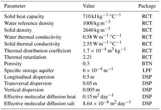
While the buoyancy flow causes energy losses, also conduction, dispersion and diffusion affect the efficiency of the ATES wells. SEAWAT (Langevin et al., 2003) not only dynamically couples MODFLOW (Harbaugh et al., 2000) and MT3DMS (Zheng and Wang, 1999) that is flow and transport (Hecht-Mendez et al., 2010; Langevin et al., 2010), but adds viscosity and density effects coupled to temperature and salt concentration. To gain insight in these intertwined mechanisms, a SEAWAT model of ATES systems in salinity stratified aquifers was set up, without neighboring wells and ambient groundwater flow. An axisymmetric SEAWAT model with a high vertical discretization was applied to simulate in detail the vertical flow components in the entire aquifer and along the well screen (Langevin, 2008; van Lopik et al., 2016). van Lopik et al. (2016) calibrated an axisymmetric model of a high temperature (80 ^∘C) ATES system against monitoring data, in which buoyancy flow was a dominating process. The model set-up and parameter values in this study follow their work, Table 3 and Fig. 4.

• Discretization. The grid applied with SEAWAT is a vertical section of one row, with distance along the columns and depth along the layers. The wells screen(s) are in different layers in the first column. A doublet is represented by 3 rows, where the two outer rows, model the warm and cold well, while the middle row was set to inactive to prevent interaction between the outer rows. The horizontal discretization is 2 m at the well face, cell size grows logarithmically with radial distance to a maximum of 250 m at the outer boundary of the model, in 50 steps. The Courant number is the ratio transport distance during one time step over the cell size (Courant et al., 1967) and should be smaller than 1 for accurate calculation. In this set-up it is larger than 1 close to the well, with an applied time step of five days, and smaller than one at several meters away from the well and onwards, where buoyancy flow, conduction, dispersion matter.

• Model layers. To allow for sufficient detail and insight in the vertical buoyancy flow component, the layers are also discretized at high resolution; 0.5 m thickness, irrespective the thickness of the aquifer that is simulated. The model can be thought of to consist of an aquifer that is confined by 10 m thick aquitards at its top and bottom. No recharge was applied. Constant head, temperature and salinity boundaries were applied at outer boundary. The inner and lower boundary at r=0 were closed. The top of the upper confining layer has a constant temperature.

  The aquifer thickness varies over the simulated scenarios. The wells screens of the doublets were always fully penetrating and those of the monowells always penetrated the top and the bottom third of the aquifer. The flow from the injection screen entering different model layers is calculated proportionally to the transmissivity of each model layer.

• Model extent and time horizon. To prevent boundary conditions from influencing simulation results, several test runs were carried out. These showed that the outcomes changed less than 1 % with the outer boundary set at 1500 m. The time horizon was set to 10 years as these test runs showed was sufficiently long to evaluate the effect of multiple years of operation until stable recovery efficiency was achieved and to fully assess the buoyancy flow impact and its dynamics.

• Parameter values. The parameter values follow van Lopik et al. (2016) adapted to axisymmetric flow according to Langevin (2008). These values are given in Table 3. The viscosity and density dependency on temperature and salt concentration was implemented following Eqs. (4) and (5). The extraction temperature and salt concentration as calculated by SEAWAT for every cell representing the well screen, are averaged in proportion to cell transmissivity. The thus computed extracted salinity is used as infiltration salinity of the coupled well screen.

• The groundwater flow was solved using the preconditioned conjugate-gradient 2 package. The standard finite-difference method with upstream or central-in-space weighting was applied in the advection package for the temperature and salt concentration simulation.

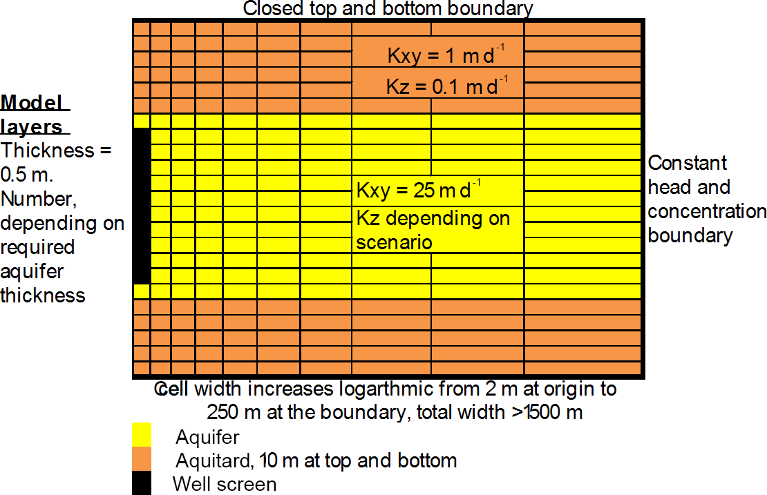
Figure 4 Schematic representation of model setup, indicating cell sizes, layers and boundary conditions.

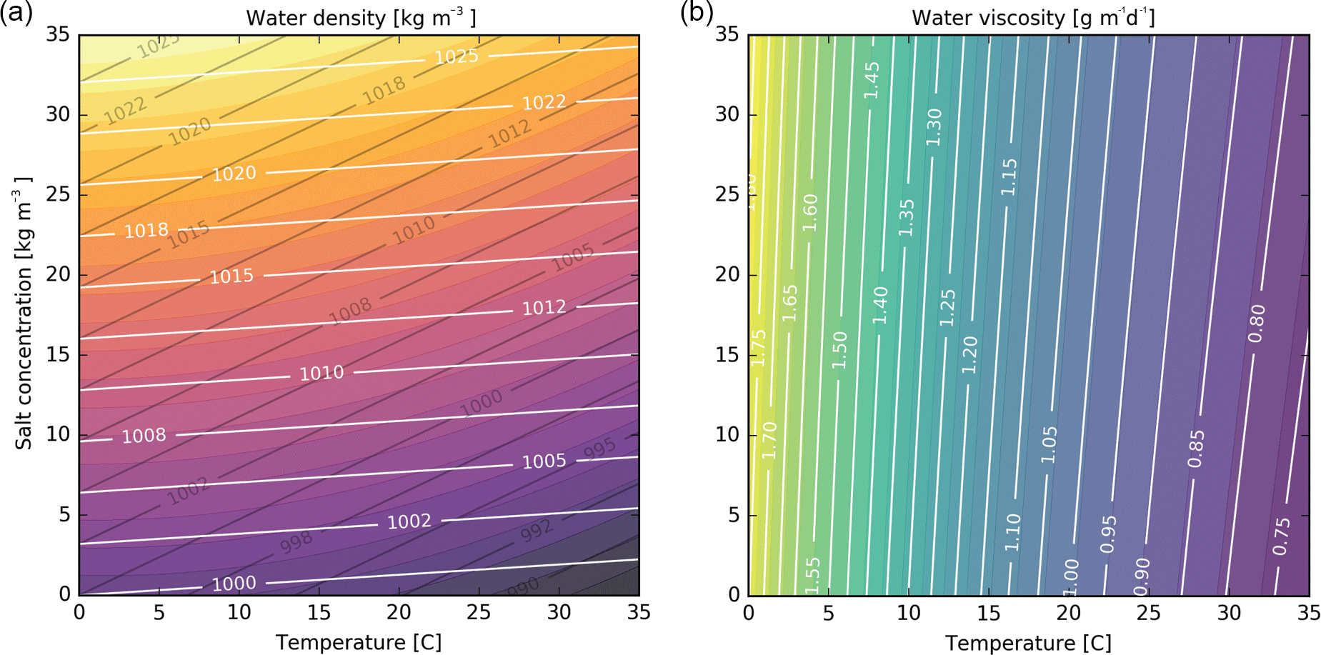
Figure 5 (a) Water density as a function of temperature and salt concentration. Color filled contours are (Sharqawy et al., 2012) grey lines: Eq. (3), white lines: Eq. (4). (b) Water viscosity as a function of temperature and salt concentration, both colored filled contours and white lines: Eq. (5).

2.4 The effect of salt concentration and temperature on density and viscosity

Both the density and viscosity of the water are functions of salinity, temperature and pressure. However, for the depth range of interest, the dependency of pressure is negligible (Sharqawy et al., 2012; van Lopik et al., 2016). The geohydrological conditions and ATES characteristics identified in the sections above are now used to determine to what extent density and viscosity are affected by changes in salt concentration and temperature. In groundwater modeling the often-used equation (Langevin et al., 2003) of state for density (ρ [kg m⁻³]) as a function of temperature and salt concentration is:

$$\begin{array}{}\text{(3)}& {\displaystyle }{\displaystyle }\mathit{\rho }(S,T)=\mathrm{1000}+\mathrm{0.78}S-\mathrm{0.375}T\end{array}$$

where T is the temperature of the water [^∘C] and S the total salt concentration [kg m⁻³] (Langevin et al., 2008; Lopik et al., 2015; Thorne et al., 2006). However, the slope of this linear approximation for the temperature influence is too steep over the range of 5 to 15 ^∘C in which ATES operate. Figure 5a shows this by plotting Eq. (3) in grey contour lines together with the non-linear density relation as described by Sharqawy et al. (2012) as shown in colored filled contours. For this study Eq. (3) is replaced by;

$$\begin{array}{}\text{(4)}& {\displaystyle }{\displaystyle }\mathit{\rho }(S,T)=\mathrm{1000}+\mathrm{0.78}S-\mathrm{0.1}T\end{array}$$

to correct the density-temperature slope for the 5 to 15 ^∘C temperature range, from −0.375 to −0.1. This yields the white contour lines in Fig. 5a. Salt concentration and temperature also affect fluid viscosity (μ [kg m⁻¹ day⁻¹]), to which the hydraulic conductivity is proportional (Fetter, 2001). The relation between viscosity, salt concentration and temperature may be approximated following Voss (1984);

$$\begin{array}{}\text{(5)}& {\displaystyle }{\displaystyle }\mathit{\mu }(S,T)=\mathrm{2.394}\times {\mathrm{10}}^{-\mathrm{5}}\times {\mathrm{10}}^{\frac{\mathrm{248.8}}{T+\mathrm{133.2}}}+\mathrm{1.923}\times {\mathrm{10}}^{-\mathrm{6}}S.\end{array}$$

Figure 5b shows that viscosity depends much stronger on temperature than on salt concentration over the range of temperature and salt concentration identified for this study. Around warm wells, flow in the subsurface is enhanced by the increased hydraulic conductivity caused by the reduction of viscosity with higher temperatures (Fetter, 2001)

This research neglects the geothermal gradient. At common values for the geothermal gradient like also present in The Netherlands (∼0.03 ^∘C m⁻¹), the density change is dominated by the increasing salt concentration. The geothermal gradient has a larger influence on the viscosity change, it is still neglected because the thermal front is retarded with respect to injected water front, the dominating buoyancy flow occurs at the injected water front, so without a significant viscosity difference.¹

3 Analytical analysis of buoyancy flow

The mechanisms involved in the heat transport are described in Sect. 2. The effect of horizontal ambient groundwater flow on the recovery efficiency of water stored in aquifers has been studied extensively (e.g. Bear and Jacobs, 1965; Ceric and Haitjema, 2005). Vertical flow components as a consequence of buoyancy flow have also extensively studied (e.g. Hellström et al., 1988; Massmann et al., 2006; Simmons et al., 2001; Ward et al., 2007). In this subsection the usability of analytical relations found in these studies is evaluated for the purpose of establishing the magnitude of buoyancy flow around ATES wells and its most important parameters.

3.1 Mixed convection ratio

Massmann et al. (2006) define the mixed convection ratio (M) to identify which processes dominate during the periods of infiltration, extraction and storage in situations where buoyancy flow is involved.

$$\begin{array}{}\text{(6)}& {\displaystyle }{\displaystyle }M={\displaystyle \frac{D}{\mathrm{\Delta }h}}{\displaystyle \frac{{\mathit{\rho }}_{\mathrm{in}}-{\mathit{\rho }}_{\mathrm{0}}}{{\mathit{\rho }}_{\mathrm{0}}}}\end{array}$$

with Δh the difference in hydraulic head between the screens of the wells [m] and D is horizontal distance between the screens [m]. The first factor in Eq. (6) is proportional to the forced convection while the second is proportional to the buoyancy. According to Massmann et al. (2006), mixed convection ratios larger than 1 indicate dominance of buoyancy flow, while M<1 indicates dominance of forced convection. This metric was used to identify to what extent buoyancy flow dominates during the storage phase only or during storage, infiltration and extraction. Because the density of the ambient groundwater varies with depth, the largest occurring density difference between injected and ambient groundwater along the well screen, was used in Eq. (6) to determine the mixed convection ratio. For monowells the vertical distance between the bottom of the top and the top of the bottom screen is used for the D in Eq. (6). The results are plotted in Fig. 6 for the full range of combinations in density gradient and vertical hydraulic conductivity defined in Sect. 2. The monowells generally have a higher mixed convection ratio, which indicates that buoyancy losses are larger for monowells than for doublets. At the largest density gradient (1 kg m⁻³ m⁻¹) the mixed convection ratios are little over 1, indicating that only under extremely large density gradient conditions the buoyancy flow may have a large impact on thermal efficiency of the ATES wells.

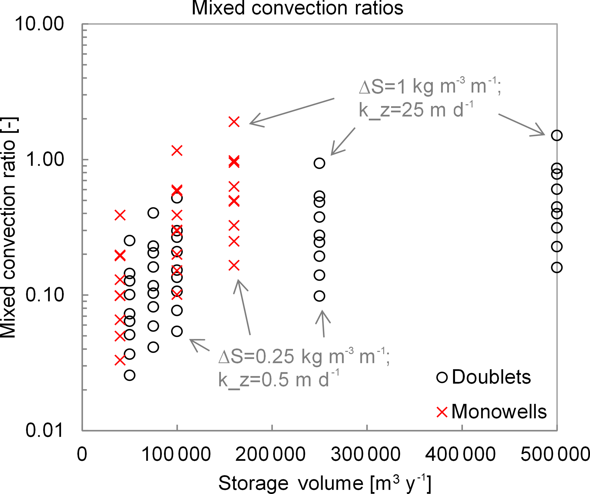
Figure 6 Mixed convection ratios for ATES systems conditions following Table 1 and Eq. (6). The head difference between the two wells was estimated conservatively to not underestimate the mixed convection ratio; for doublets 10, 7 and 5 m, for monowells 6, 4 and 2 m for k-values of 0.5, 10 and 25 m day⁻¹ respectively. The distance between the well for doublets is set to 3R_th, and 1L for monowells.

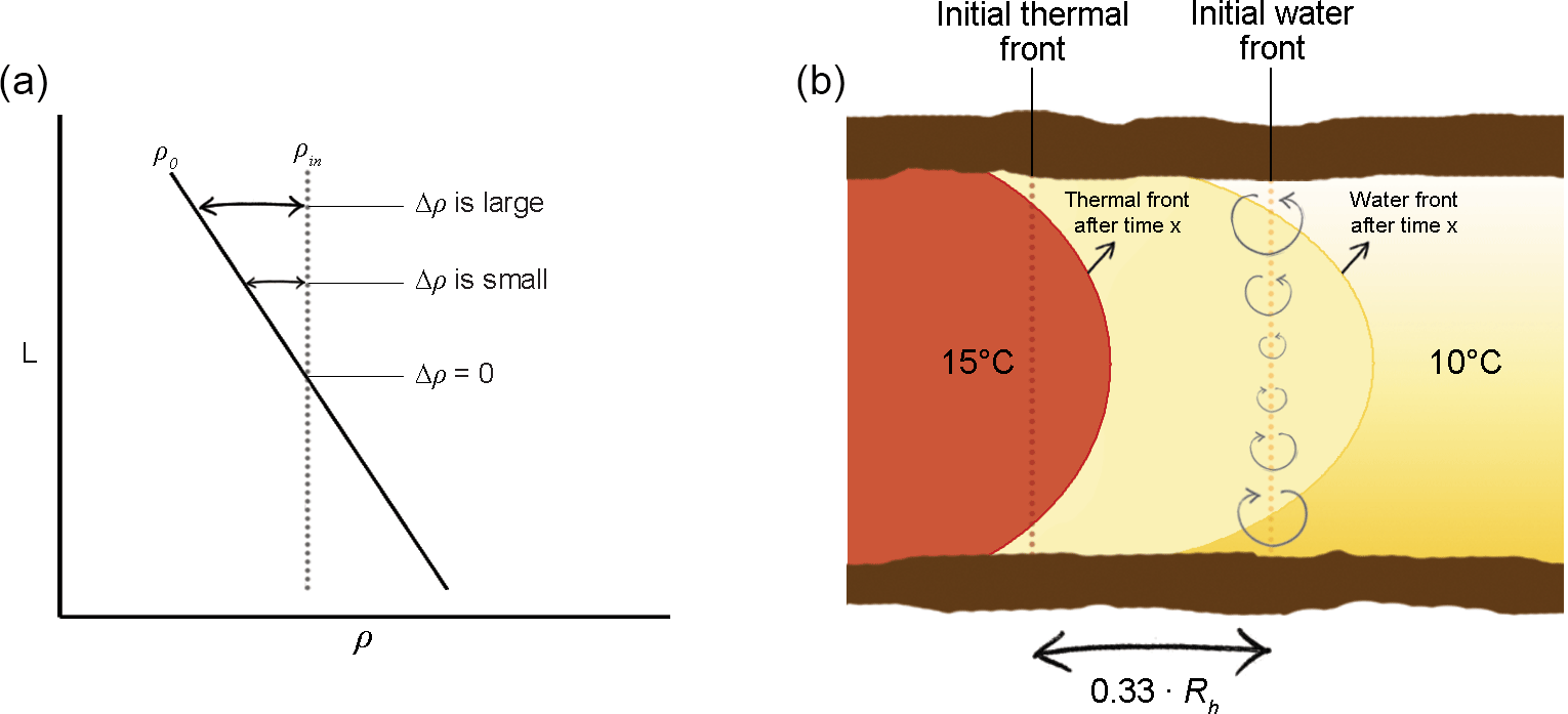
Figure 7 (a) Schematic representation of the differences in density of injected and ambient groundwater along the screen (L). (b) Schematic representation of development of tilting along an interface between infiltrated water with a constant density in an aquifer with a density gradient along aquifer depth. The initial thermal front is the thermal radius (Eq. 2), the extend of the infiltrated water is the hydraulic radius (R_h) which is about 1.5 times larger than the thermal radius (Bloemendal and Hartog, 2018).

3.2 Characteristic tilting time of the density difference interface

Because the density-forced tilting of the interface between the injected and ambient groundwater continues until the equilibrium situation is reached, the time this tilting process takes relative to the storage cycle length is an important measure to identify how strong the losses due to buoyancy flow are. Hellström et al. (1988) derived an expression that quantifies the characteristic tilting time of an axially symmetric interface between fresh and salt water:

$$\begin{array}{}\text{(7)}& {\displaystyle }{\displaystyle }{t}_{\mathrm{0}}={\displaystyle \frac{\mathrm{1}}{{\mathit{\omega }}_{\mathrm{0}}}}={\displaystyle \frac{c_{\mathrm{aq}}}{c_{\mathrm{w}}}}{\displaystyle \frac{L}{\sqrt{{\mathit{\kappa }}_{\mathrm{h}}{\mathit{\kappa }}_{\mathrm{v}}}}}{\displaystyle \frac{{\mathit{\pi }}^{\mathrm{2}}\left({\mathit{\mu }}_{\mathrm{0}}+{\mathit{\mu }}_{\mathrm{1}}\right)}{\mathrm{32}Gg\left({\mathit{\rho }}_{\mathrm{0}}-{\mathit{\rho }}_{\mathrm{1}}\right)}}\end{array}$$

with ω₀ the initially vertical front rotation angular velocity, t₀ the characteristic tilting time [s], κ_h and κ_v the horizontal and vertical aquifer permeabilities [m²], μ₀ and μ₁ the viscosities of the ambient and the injected water [kg m⁻¹ s⁻¹], ρ₀ and ρ₁ the densities of the ambient and the injected water, G the Catalan's constant² [0.916] and g the gravitational constant [9.81 m s⁻²]. However, due to three aspects, this relation is not completely valid for calculating the tilting time of the injected water or thermal front in the case of ATES systems;

1. At the condition of interest, the initial ambient density increases linearly with depth and, therefore, also across the interface between the injected and ambient groundwater, while Hellström et al. (1988) assume homogenous ambient density. Due to the ambient density gradient, it is expected that rotation of the interface varies with aquifer depth because the density difference between injected and ambient water increases towards both the top and the bottom of the aquifer (Fig. 7a), which results in increasing rotation speeds towards the top and bottom of the aquifer. This increasing rotation speed towards the top and bottom of the aquifer results in a curved interface between injected and ambient groundwater, see Fig. 7b. For this study, the largest density difference at the top and bottom of the aquifer is used to compute the tilting times with Eq. (7). This results in an overestimation of the average characteristic tilting time of the water interface.

2. Hellström et al. (1988) assume that the interface of density difference coincides with that of viscosity, but around an ATES well the jump in viscosity is at the thermal front, which lags behind the water front, as can be seen from Figs. 5b and 7b. The computed tilting times are, however, not corrected for this thermal retardation effect, which results in an underestimation of the characteristic tilting time of the front of the injected water.

   The tilting at the thermal interface is less strong than at injected water front because the buoyancy flow components decline with distance to injected water front. According to Hellström et al. (1988) the width (w_c) of a free convection cell around the tilting interface is the aquifer thickness (L) over the anisotropy factor (a_v). The amount of decline is expressed by the ratio (d_r) of the width of the free convection cell over the distance between the thermal and the injected water front (0.33R_th, Eq. 2):

   $$\begin{array}{}\text{(8)}& {\displaystyle }{\displaystyle }{d}_{\mathrm{r}}={\displaystyle \frac{w_{\mathrm{c}}}{\mathrm{0.33}{R}_{\mathrm{th}}}}.\end{array}$$

   This distance ratio (d_r) expresses the extent to which the thermal front lies within the convection cell of the injected water front. When d_r is close to 1 the tilting is strongly excersized on the thermal front, when it is close to 0 the thermal front is hardly affected by buoyancy flow.

   For small storage volumes and/or long screen lengths, the tilting of the injected water front affects tilting of the thermal front stronger than in the case of large storage volumes and/or short screens. In the case of a sufficiently large thermal radius relative to the aquifer thickness, the width of the free convection cell may become smaller than 0.33R_th, in which case tilting of the thermal front will not occur at all. With anisotropy factors ranging from 2 to 10 and aquifer thicknesses from 10 to 150 m, the widths of the free convection cells that occur around ATES wells vary between 1 to 150 m.

3. Due to thermal retardation, any tilting of the thermal interface rotates at about half the speed of the tilting rate of the water front.

3.3 Discussion analytical analysis

Despite the limited validity of Eqs. (7) and (6), it is still valuable to get an indication of the order of magnitude of the expected buoyancy flow due to a vertical density gradient during a typical ATES storage-cycle. Despite the limited validity, it is concluded that, at high vertical conductivity combined with a large ambient salinity gradient, the buoyancy flow may affect ATES efficiency, especially for monowells.

The characteristic tilting times calculated, are initial tilting times, which progressively increase. So, at a characteristic tilting time equal to, or smaller than the storage period, heat loss due to buoyancy can be considerable. Storage periods of ATES systems last typically about a quarter year, so that with characteristic tilting times of 90 days or shorter, buoyancy flow may considerably reduce the recovery efficiency of ATES wells.

Table 4 Characteristic tilting times (t₀) of water interface of two different densities, following Eq. (7), corrected for heat retardation. The screen lengths (L) follow the corresponding values of Table 1. Maximum ratio of width (d_r) of the free convection cell and distance between water and thermal front. Distance ratio values > 1 indicate that the buoyancy at the water front affect the thermal front. The range of conditions included originate from the ones identified in Table 1, k_z = vertical conductivity, L = screen length, V = storage volume, ΔS = salinity gradient. Bold numbers: conditions under which buoyancy flow may have a considerable effect on recovery efficiency.

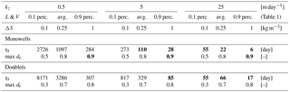
The obtained tilting times are presented in Table 4, together with the values of the distance ratio (d_r) for the range of conditions identified in Tables 1 and 2. The identified tilting times (t₀) and distance ratios (d_r) show that buoyancy flow may have a considerable effect on recovery efficiency at only some of the most extreme conditions (bold font in Table 4), i.e. combination of high conductivity, large density gradient and long screens. In general buoyancy has a stronger impact on monowells, due to the larger density differences as a consequence of the position of the screens in the top and bottom of the aquifer.

Similarly, the monowells generally have a higher mixed convection ratio, which indicates that buoyancy losses are larger for monowells than for doublets. At the largest density gradient (1 kg m⁻³ m⁻¹) the mixed convection ratios are little over 1, indicating that only under extremely large density gradient conditions the buoyancy flow may have a large impact on thermal efficiency of the ATES wells.

4 Numerical simulation of buoyancy flow

The analytical solutions only take into account the initial situation and disregard feedbacks of the spreading of dissolved salt and heat with time propagating over multiple storage cycles. In this section, numerical simulations are used to study such propagation effects over several ATES cycles. These simulations also quantify the effect of buoyancy flow on the recovery efficiency as well as the effects of mechanical dispersion and conduction. This is done for the ranges in monowell and doublet systems and geohydrological conditions identified in Sect. 2. The losses are compared to those under the same circumstances, but with a constant density in the aquifer. Before various ranges on conditions are simulated in Sect. 4.2 and 4.3, first a case study is simulated to get a better understanding and insight in practical and real life conditions.

Table 5 Monowell characteristics provided by ATES contractor Installect B.V.

4.1 Case study Amsterdam

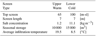
To also include practical aspects in this evaluation, design and monitoring data were obtained for a monowell system in the city of Amsterdam. The local density gradient of 0.28 kg m⁻³ m⁻¹ was derived from water-quality samples taken at the installation, see Table 5. Xynogalou (2015) found an anisotropy of 8 for the aquifer below Amsterdam boiling down to a vertical hydraulic conductivity of 6 m day⁻¹ with some variations at different depths, which is consistent with earlier work from Caljé (2010).

The axisymmetric model was adapted to the conditions for this monowell system and simulated for the situation with and without the ambient density gradient. Because the two screens are relatively far apart and short, also scenarios were simulated where screens are twice as long (14 m) and placed closer together (20 m instead of 28 m). Thick aquifers like the one used in this case are often intersected by thin clay layers. The effect of such layers was also explored by adding a 2 m thick clay layer between the two wells. The first two simulation results in Table 6 show that for the situation as installed, the density gradient in the aquifer under Amsterdam does not affect the efficiency much.

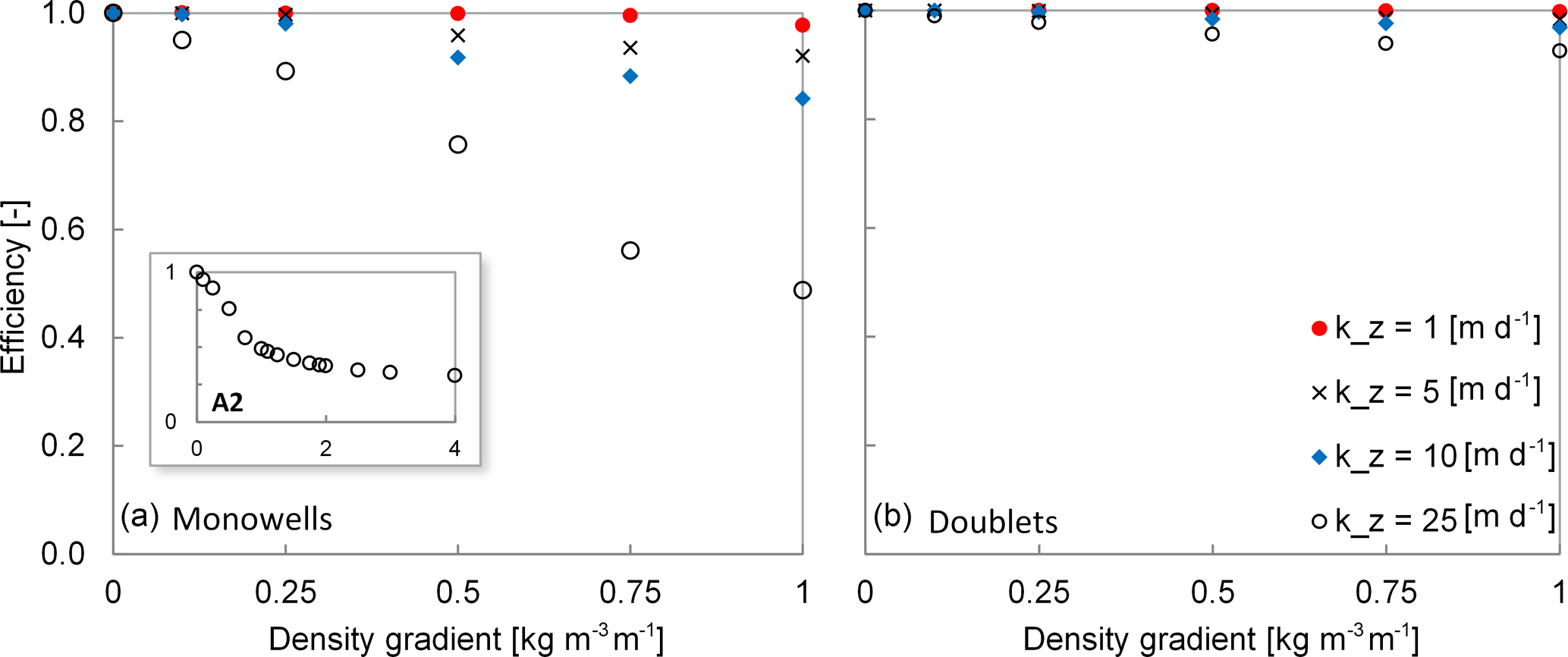
Figure 8 The average recovery efficiency after 10 year simulation period as a function of density gradient and different geohydrological properties, for average sized (a) Monowell and (b) Doublet systems.

Table 6 Average extraction temperatures and overall efficiency of the 3 year simulation of the case study ATES system at different alternative well designs and aquifer conditions. Screen spacing as function of the screen length (L).

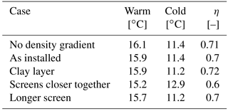
Adding a thin clay layer in between the screens results in an overall efficiency improvement, due to the improved thermal efficiency of the cold screen. Following the mechanisms discussed in this section it can be expected that in this case the warm screen suffers from the largest buoyancy flow, which hardly depends on a clay layer in between the screens. This clay layer prevents the heat from moving close to the cold screen, which results in an improved efficiency of the cold screen.

The two cases with the altered screens (last two lines in Table 6) suggest that the short-circuit flow between the two screens has a larger effect on efficiency than the losses due to buoyancy flow. In the previous subsection, the spacing between the screens was kept the same as the screen length. The effect of the distance between the screens was evaluated, for several scenarios described in Table 7, for a monowell with average storage volume. The results in Table 7 confirm that short-circuit flow between the two screens has a larger influence than the buoyancy.

4.2 Impact of the aquifer's density gradient on ATES efficiency

4.2.1 Monowells

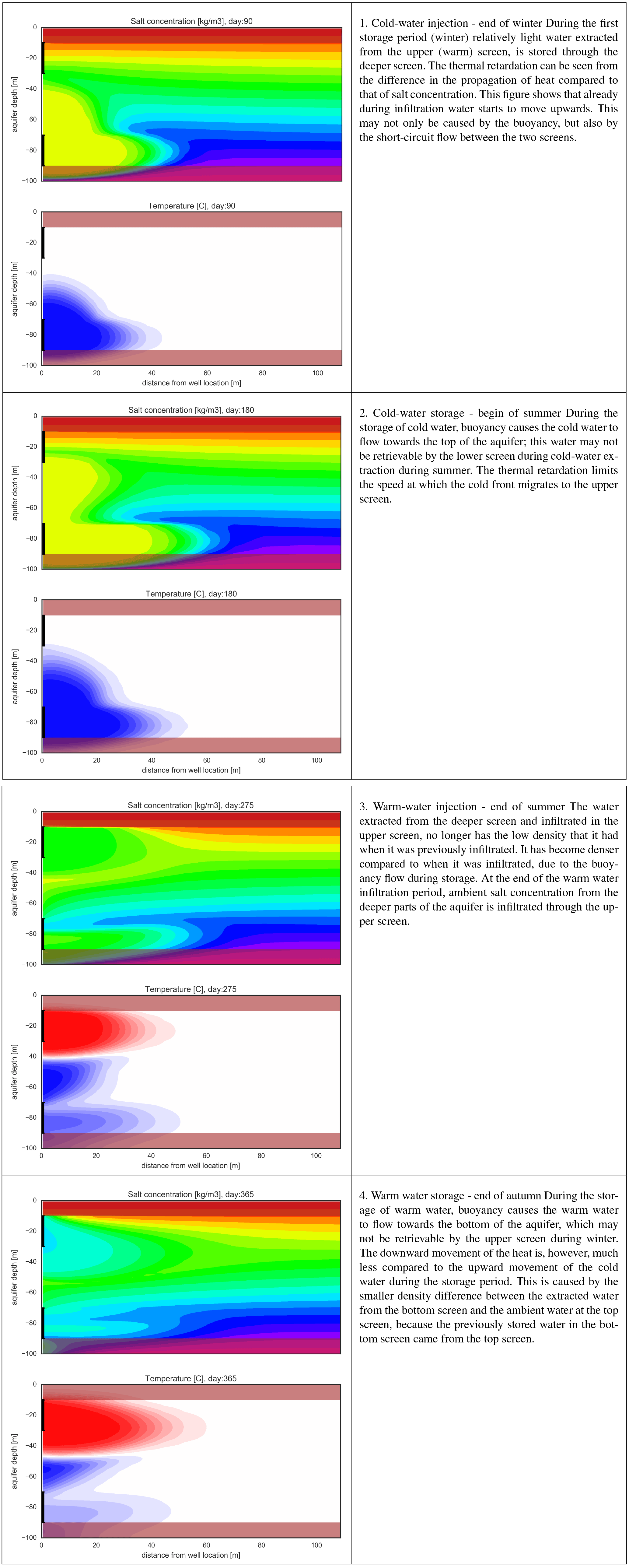
Table A1 shows the density and temperature distribution around an average-sized monowell at 4 moments in the first year of operation, these figures are used to discuss the processes of buoyancy flow and heat loss around the monowell screens.

The average recovery efficiencies of both warm and cold screens after 10 cycles are shown in Fig. 8a for different vertical conductivities as a function of the vertical salinity gradient. The losses due to buoyancy flow are negligible for small vertical hydraulic conductivities and/or small salinity gradients, while the losses increase for increasing salinity gradients and vertical conductivities, reaching over 50 % under the most extreme conditions. In all scenarios, the recovery efficiency stabilizes after 4 to 6 storage cycles.

Table 7 Average extraction temperatures and overall efficiency of the 3 year simulation of the average Monowell system at different alternative well spacing distances and aquifer conditions. V = 100 000 m³ y⁻¹, k_z = 6 m day⁻¹. Screen spacing as function of the screen length (L).

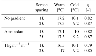
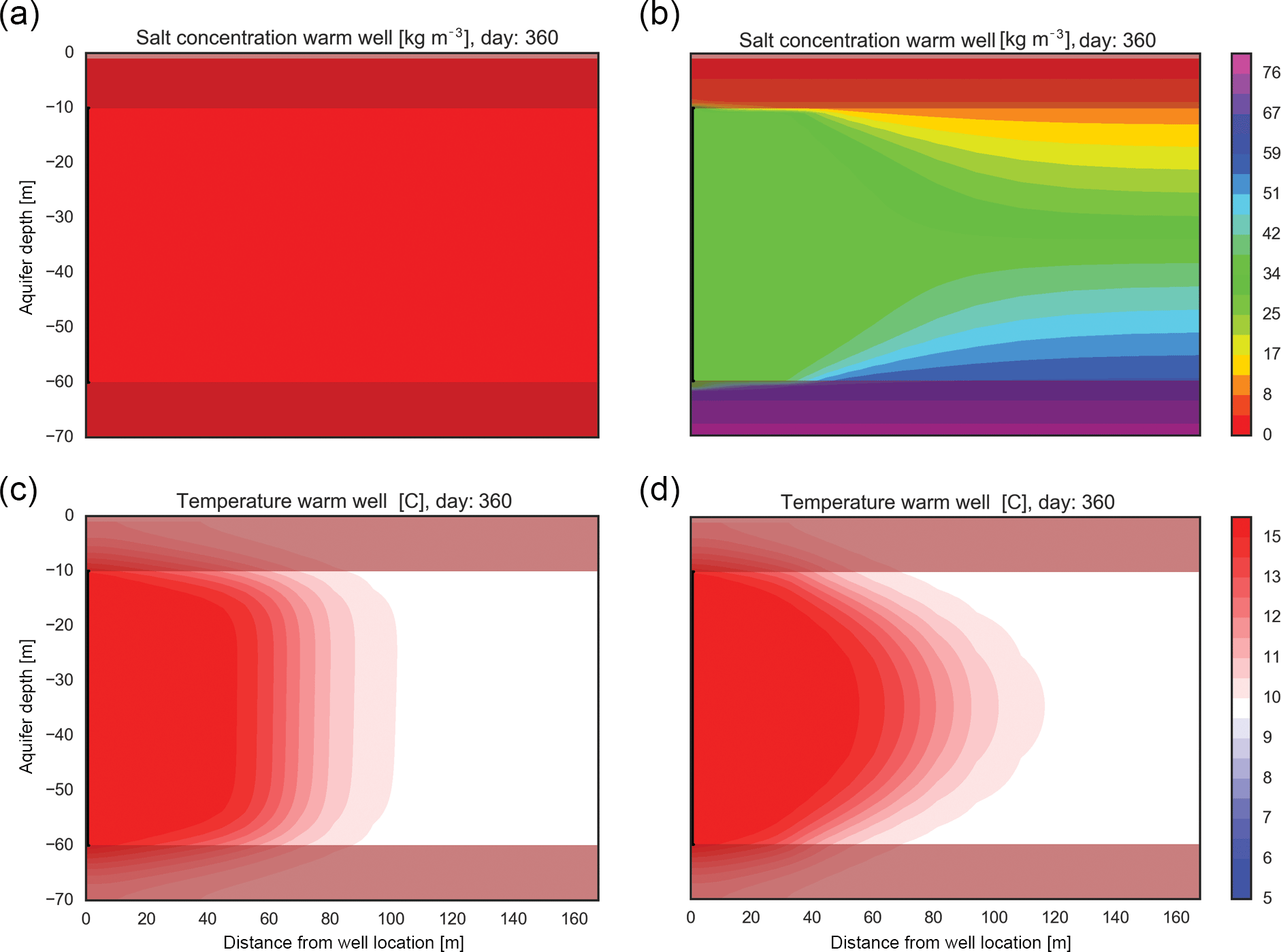
Figure 9 Cross-sectional overview of density (a, b) and temperature (c, d) distribution after one year of operation of a warm well, k_z=10 m day⁻¹, storage volume = 250 000 m³, fully penetrating screen located on the y-axis at 10–60 m-sl. (a, c) No density gradient, (b, d) a gradual density gradient of 1 kg m⁻³ m⁻¹.

The short description and cross sections shown in Table A1 are now used to discuss the relations shown in Fig. 8a. The relations in Fig. 8a can be best explained following the discussion in step 2 of Table A1: The ambient vertical density gradient and the vertical conductivity determine the extent at which the infiltrated water is affected by buoyancy flow. In the example in Table A1, both are relatively large, which results in strong upward flow during cold-water storage and also in strong downward flow during warm-water storage. But when the vertical conductivity and ambient density gradient are small, then during cold-water storage, buoyancy flow is low, and the extracted water from the lower screen during summer has a density that is still much closer to the ambient density at the upper screen, which results in smaller changes of the density differences during storage in the upper screen and fewer losses than is the case in Table A1 (step 4).

This discussion explains why in Fig. 8a the relation between efficiency and ambient density gradient has a flat slope when the vertical conductivity is small. At first, the losses at the both screens remain limited, but become aggravated as the conductivity and density gradient continue to increase, which results in a steeper slope. This can be seen in Fig. 8a for the simulation results with k_z=25 m day⁻¹. For the case k_z=25 m day⁻¹, simulations were carried out for (hypothetical) ambient density gradients up to 4 kg m⁻³ m⁻¹ just to show how the relation between ambient density gradient and efficiency propagates beyond 1 kg m⁻³ m⁻¹ (see sub-plot A2 in Fig. 8). The flattening of the slope of the efficiency versus density gradient with higher ambient density gradients in Fig. 8 (A2) is caused by the following mechanism: the upward movement of the light water (yellow in step 2 of Table A1) injected in the lower screen can only reach the lower part of the upper screen, because ambient groundwater of a higher density (green in step 2 of Table A1) enters the middle part of the upper screen.

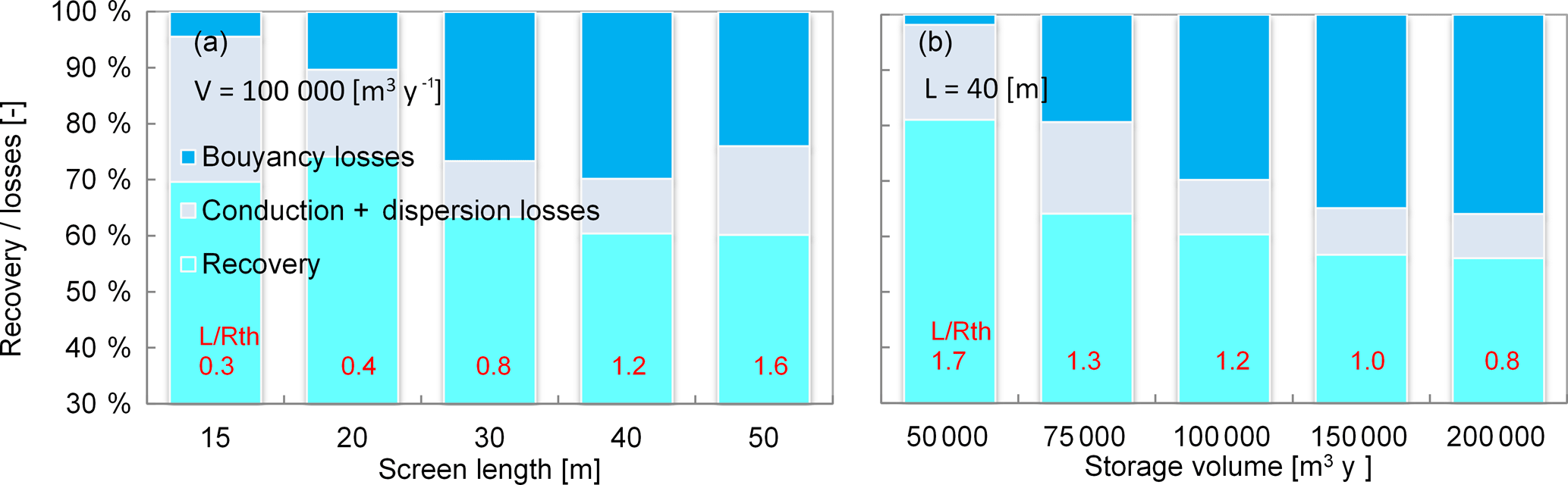
Figure 10 Heat recovery, buoyancy, conduction anddispersion losses, relative to monowell design and storage volume at 1 kg m⁻³ m⁻¹ density gradient and vertical conductivity of 10 m day⁻¹. Short circuit flow between wells contribute to losses as well, those could not be separated from the results. At the smallest screen lengths and largest storage volumes the conduction and dispersion part is likely to also contain the losses to short circuit flow. This also explains the low recovery efficiency in those cases.

4.2.2 Doublets

Both wells of the doublet usually have their screen at the same depth. Therefore, their thermal energy losses are equal. The efficiency of both the warm and the cold well over 10 cycles are shown in Fig. 8b. The figure shows that also for doublets, both the vertical conductivity and vertical density gradient affect the losses due to buoyancy, however, less strongly than for monowells. Also, all doublet wells reach stable recovery efficiencies after 4 to 6 cycles. The results of these numerical simulations did not show any considerable changes in the maximum extent of thermal radius over the 10-cycle simulation period. Figure 9 shows the density and temperature distribution around the warm well after the first warm-water storage period for both 0 and 1 kg m⁻³ m⁻¹ ambient density gradients. Figure 9d confirms the gradual tilting of the thermal front that was discussed in Sect. 2 and schematically indicated in Fig. 7.

4.3 The effect of well design on buoyancy losses

Next to buoyancy flow, the spreading of heat by conduction and dispersion at the boundary of the thermal cylinder and advection by groundwater flow are the dominant processes that cause energy to be unrecoverable for the ATES well (Anderson, 2005; Bloemendal and Hartog, 2018; Caljé, 2010). Different design strategies are now evaluated to firstly identify the relative contribution of conduction, dispersion and buoyancy losses and secondly, to identify possible controls to maximize overall efficiency.

Doughty et al. (1982) and Bloemendal and Hartog (2018), use the ratio of screen length over thermal radius (L∕R_th) as a design criterion to ensure maximum heat-recovery efficiency. They found that this ratio should be between 1 and 4. Next, it is identified what values of this L∕R_th-ratio lead to optimal well design when buoyancy flow contributes to the heat losses. The contribution of buoyancy to the heat losses is investigated by simulating scenarios with and without a vertical density gradient. The increase of dispersion caused by buoyancy flow is considered negligible.

Earlier in this section it was shown that the losses due to a vertical density gradient are only important when both this gradient and the vertical hydraulic conductivity are high. Therefore, the relative influence of conduction, dispersion and buoyancy is considered only at the maximum ambient density gradient of 1 kg m⁻³ m⁻¹ and vertical conductivity of 5 m day⁻¹ for the range of ATES system sizes and screen lengths indicated in Table 1. The average ATES system size is used as a base case and altered systematically over the ranges identified in Sect. 2.

4.3.1 Monowells

Figure 10 shows the simulation results. Distinction is made between the recovery of heat on the one hand and losses due to conduction-dispersion and buoyancy on the other.

Figure 10a shows the result of a stepwise increase of the screen length for a constant storage volume. Simulations for other storage volumes are not shown because the results show the same trend. The smallest screen length yields the smallest buoyancy losses because the density difference between the upper and the lower screen is then smallest. N.B. the screen length of the simulated monowell is one third of the aquifer thickness. Therefore, small screens imply smaller density differences both at and between the screens. The conduction and dispersion losses are large because of the low L∕R_th-ratio, which results in large conduction losses to the confining layers.

With the stepwise increase of the screen length, Fig. 10a shows that at the first steps, the buoyancy losses increase due to the greater density differences between the upper and the lower screen. The conduction and dispersion losses become smaller due to the increased L∕R_th-ratio, which reduces the total area of the circumference of the heat volume in the aquifer and thus the losses due to conduction and dispersion.

At the largest well-screen lengths conduction and dispersion losses increase again, where the optimum L∕R_th-ratio is exceeded. For the smallest storage volume conduction and dispersion even dominate the buoyancy losses.

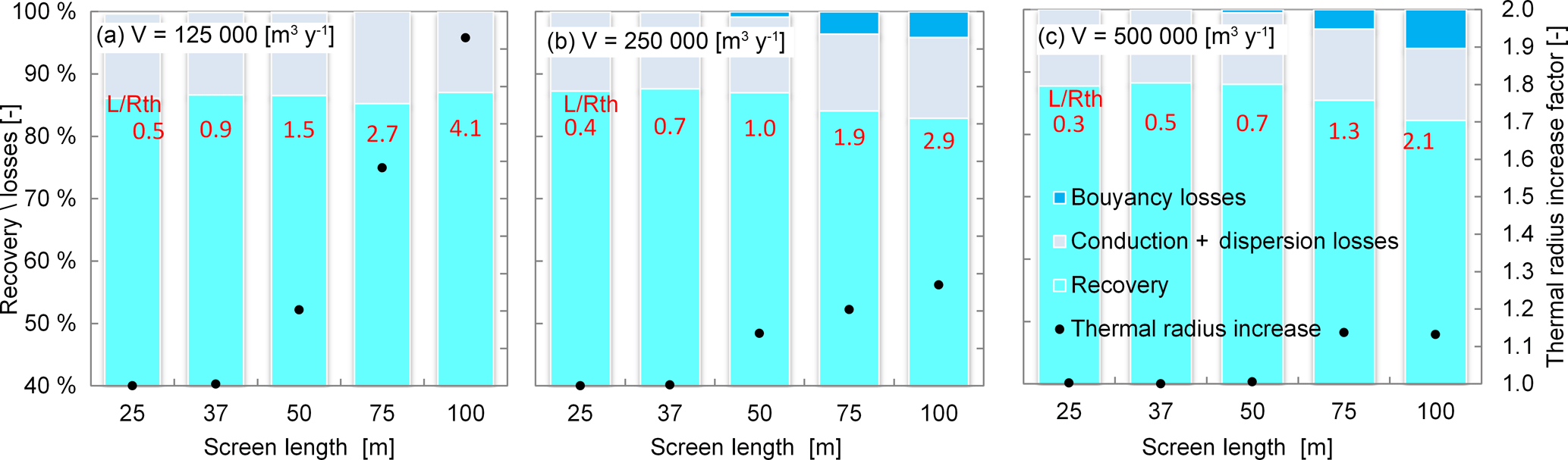
Figure 11 Heat recovery, buoyancy and conduction anddispersion losses, relative to doublet well design and storage volume at 1 kg m⁻³ m⁻¹ density gradient and vertical conductivity of 10 m day⁻¹.

In situations without a density gradient, increasing the storage volume results in a higher efficiency. Remarkable is the observation that recovery decreases with increasing storage volume as shown in Fig. 10b. This is explained by the fact that at larger storage volumes more heat can flow towards the other screen. Because the thermal radius is larger, any vertical buoyancy flow results in larger heat losses. With same the well-screen length an increasing storage volume, also the short-circuit flow increases. For monowells, larger storage volumes are more sensitive to losses caused by buoyancy flow and short-circuit flow than to dispersion and conduction. Despite the lower relative dispersion and conduction losses expected at larger storage volumes, larger storage volumes may lead to lower recovery rates than smaller storage volumes in these specific conditions.

Both the losses due to buoyancy and those due to conduction are strongly affected by the applied length of the screens of the monowells. For short screens, dispersion and conduction losses are largest as a result of large conduction losses to confining layers. For the longest screens, buoyancy losses generally dominate because then density differences between the top and the bottom screen are larger. The highest efficiency is attained for intermediate screen lengths, where neither type of losses dominates.

4.3.2 Doublets

Similar to the monowells, longer well screens cause larger buoyancy losses for doublets (see Fig. 11). For doublets, the buoyancy flow does not affect efficiency as much as for monowells. The small buoyancy losses that characterize doublets, also limit the increase in thermal radius that is caused by the buoyancy flow. Counter-intuitively, the increase in thermal radius is only considerable for the smallest storage volume (Fig. 11a), with its characteristic high ratio of screen length over thermal radius. The buoyancy-induced change in thermal radius is more or less constant over the range of simulations carried out for doublets; it varies from hardly noticeable for a short screen, to about 15 m for the longest screen (100 m).

5 Discussion

Well design can help reduce heat losses caused by buoyancy flow; a longer screen increases the density differences between upper and lower (part of the) screens, thus aggravating buoyancy losses. This is, however, compensated for by a smaller thermal radius, which limits these buoyancy losses, especially for monowell systems. To obtain the highest recovery efficiency, the results indicate that in case of buoyancy flow, the optimal L∕R_th-ratio has to be chosen smaller than the thresholds identified by Doughty et al. (1982) and Bloemendal and Hartog (2018). For monowells it is more important to prevent short-circuit flow between the screens, which requires sufficient spacing between the top and bottom screen.

In coastal aquifers ambient (lateral) groundwater flow is usually very limited, thus not affecting the processes discussed in this paper. However, in areas with extraction or with a steep groundwater head gradient resulting in a groundwater flow velocity of (e.g.) >25 m yr⁻¹ (Bloemendal and Olsthoorn, 2018), the ambient groudwater flow would then dominate over the losses due to the vertical density gradient.

6 Conclusions

This study included a wide range of geohydrological conditions, and shows that within the conditions pertaining to coastal aquifers in the Netherlands (described in Sect. 2), an ambient vertical density gradient has a negligible effect on the thermal recovery efficiency of ATES systems. An ambient density gradient of over 0.5 kg m⁻³ m⁻¹, combined with a vertical conductivity over 5 m day⁻¹, has a considerable impact on the efficiency of monowell ATES systems, but these do not occur in the Netherlands.

The largest vertical ambient density gradient of 1 kg m⁻³ m⁻¹ evaluated in this research, leads to a groundwater density that exceeds seawater density in the lower part of aquifers with a thickness larger than 35 m. Although groundwater with salinities of several times that of seawater also occurs in parts the Netherlands at depths larger than 1000 m, this is not the case for the shallow aquifers used for ATES. Therefore, it is not likely to encounter considerable thermal energy losses due to buoyancy flow in low-temperature ATES practice in brackish or saline aquifers in the Netherlands, as well as other coastal areas.

The thermal losses due to buoyancy for monowells affect recovery efficiency by more than 5 % at a vertical density gradient over 0.5 kg m⁻³ m⁻¹ combined with a vertical hydraulic conductivity over 5 m day⁻¹. Doublets are not sensitive to heat losses caused by buoyancy flow, even under the most extreme conditions is the efficiency decrease less than 10 %. Within the conditions pertaining to the Netherlands, buoyancy losses caused by a vertical ambient density gradients are negligible for both monowells and doublets.

Appendix A

Table A1 Cross-sectional overview of density and temperature change for a monowell with: storage volume = 100 000 m³, vertical conductivity = 10 m day⁻¹, density gradient = 1 kg m⁻³ m⁻¹, the screens are located on the y-axis; top 10–30 m-sl, bottom 50–70 m-sl. N.B.: the relatively large vertical conductivity causes the infiltrated water to also move in between the two wells due to short circuit flow during simultaneous infiltration and extraction. The color scheme is for the same as for Fig. 9: salinity gradient for the top figures, and red for warm and blue for cold in the bottom figures.