Empirical growth models for the renewable energy sector

Three simple, empirical models for growth of power consumption in the renewable energy sector are compared. These are the exponential, logistic, and power-law models. The exponential model describes growth at a fixed relative growth rate, the logistic model saturates at a fixed limit, while the power-law model describes slowing, but unlimited, growth. The model parameters are determined by regression to historical global data for solar and wind power consumption, and model projections are compared to scenarios based on macroeconomic modelling that meet the 2^∘ target. It is demonstrated that rational rejection of an exponential growth model in favour of a logistic growth model cannot be made from existing data for the historical evolution of global renewable power consumption y(t). It is also shown that the logistic model yields saturation of growth at unrealistic low levels. The power-law growth model is found to give very good fits to the data through the last decade, and the projections align very well with the scenarios. Power-law growth is equivalent to the simple law that the relative growth rate $y^{\prime }/y$ decays inversely proportional to time. It is shown that this is a natural model for growth that slows down due to various constraints, yet not experiencing the effect of a strict upper limit defined by physical boundaries. If the actual consumption follows the power-law curve in the years to come the exponential-growth null hypothesis can be correctly rejected around 2020.

1 Introduction

It is widely recognised that economic growth in most sectors finally will have to come to an end due to the constraints imposed by planetary boundaries and that we need a new paradigm in Earth System science that integrates the physical, biological, economic, social and cultural forces (Donges et al., 2017). This idea has been developed for instance in the numerous reports to the Club of Rome, starting with the seminal book “The Limits to Growth” in 1972 (Meadows et al., 1972), which contains interesting reflections on the Earth system limits to exponential growth. Later reports like the forty-year follow up, “2052: A Global Forecast for the next Forty Years” (Randers, 2012), draw rather pessimistic pictures of our energy future. Somewhat more optimistic are the 450 scenario of the International Energy Agency (IEA, 2016) and the REmap scenario of the International Renewable Energy Agency (IRENA, 2018b). These scenarios represent emission pathways that give a fair chance of limiting global warming to 2 ^∘C relative to preindustrial global mean surface temperatures.

Energy production and distribution is the sector on which everything else depends, and despite steady advances in energy efficiency, the growth of the world economy relies on continuing growth of energy consumption. Without a massive deployment of carbon capture and storage (CCS) and other negative emission technologies, the target of global warming below 2 ^∘C from preindustrial temperatures requires radical reduction of coal in electricity production over next decades (Hansen et al., 2017a; IPCC, 2014). At present there is doubt about the technical and economic feasibility of capturing and storing 4 Gt CO₂ annually by 2040. This is more than 10 % of the emissions from fossil fuels and industry, and will require thousands of large-scale CCS plants (Global CCS Institute, 2015; Le Quéré et al., 2016). The known reserves of conventional oil and natural gas will set strict limitations to the growth in the consumption of these fuels, although fracking technologies will extend their time window somewhat (IPCC, 2014). In theory, large scale implementation of fourth generation nuclear power with a total reformation of the nuclear industry and the national and international regulatory systems, could buy some time (Makabe, 2017), but the political feasibility of such a project is highly questionable. Most integrated assessment models (IAMs) used in IPCC (2014) include optimistic assumptions on implementation of negative emission technology, but still the majority of such models conclude that a future growth rate of 1–2 % of world gross domestic product constrained by the 2^∘ global temperature target will require that solar and wind power production and consumption continues to grow at present rates without fundamental constraints (Nordhaus, 2013). A fourth option, geoengineering, has not been seriously implemented in the IAMs yet, since these are the least matured set of technologies, and associated with profound ethical issues. Thus, the rather depressing state of affairs is that the prospect of meeting the IPCC temperature targets rests on the economic feasibility of accelerating growth of world-wide, large-scale deployment of at least one of four classes of technologies; CCS, 4th generation nuclear, geoengineering, or renewables, and it is by no means obvious that any of them can meet the world's demand for clean, safe, and affordable energy.

The present paper has focus on the possible constraints on the growth of the intermittent power sources; solar and wind. Consumption of hydropower and traditional bioenergy are considerably larger at present, but their growth potential is almost exhausted. For hydro this is true in the developed world, while some developing countries still have large unexploited resources. The installed capacity of hydro has doubled over the last thirty years, and the growth looks more linear than exponential. In contrast, solar and wind have been growing exponentially with a doubling time of 2 years for solar and three years for wind (IRENA, 2018b; WEC, 2016).

The continued exponential growth is compared to the IEA 450 scenario and the IRENA REmap scenario in Fig. 1a. The figure shows projected exponential growth of consumption of solar and wind power obtained by fitting a linear model to the logarithm of the consumption time series for the period 1997–2016. The red curve is solar power, the blue is wind power. The relative growth rate is $y^{\prime }/y=\mathrm{0.35}$ for solar and $y^{\prime }/y=\mathrm{0.23}$ and for wind, which lets solar power overtake wind as the leading technology before 2030. The red points to the right in the figure represent the total solar photovoltaic (PV) power consumption in 2025 and 2040 according to IEA's 450 scenario and the REmap projection of solar PV in 2050. The blue points to the right show the same data for wind power. The figure illustrates that with continued exponential growth solar and wind together can deliver enough to fulfil the 2^∘ target demands for 2050 more than twenty years ahead of time. This observation does not give us a great reason for optimism, though. It rather suggests that the era of exponential growth will soon be over.

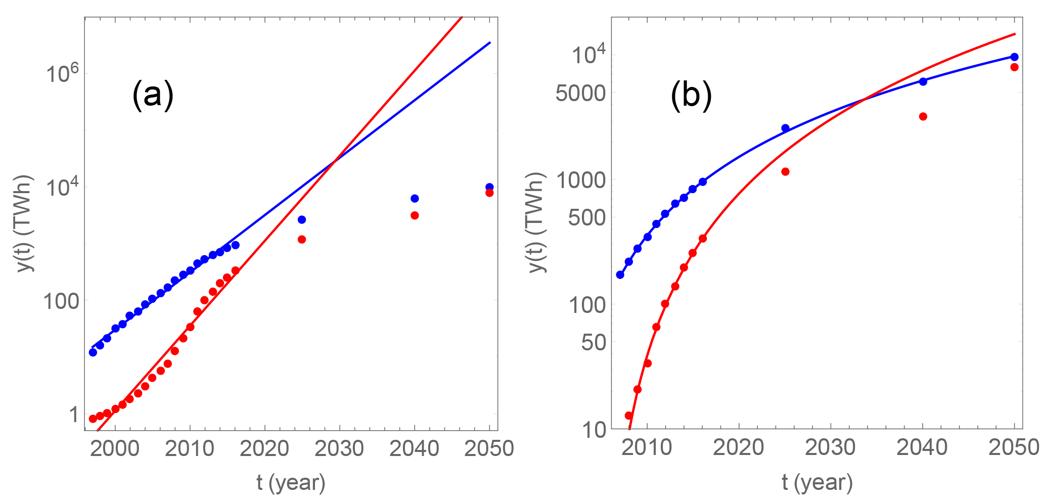
Figure 1 (a) Projected exponential growth of consumption of solar and wind power obtained by fitting a linear model to the logarithm of the consumption time series (the points to the left) for the two decades 1997–2016. Note that the vertical scale is logarithmic, so exponential growth is represented as a straight line.The red curve is solar PV power and the blue is wind power. The the red points to the right in the figure are the projected solar PV power consumption in the IEA 450 scenario for 2025 and 2040 and in the IRENA REmap scenario for 2050. The blue points to the right are the corresponding for wind power consumption. (b) The points are the same as in panel (a), but the lines are power-law fits to the points for the decade 2007–2016 for wind power and 2008–2016 for solar power.

Forthcoming sections will discuss two alternative growth models, one is the logistic model which describes initially exponential growth that saturates and finally stabilises at a fixed limit. The other is a power-law model, which does not saturate, but yields slower that exponential growth that provides a description more in line with the 2^∘ scenarios. Results of power-law fit to the historical global consumption data are shown in Fig. 1b. The fit to the wind consumption curve matches perfectly the wind consumption projections in the 450 scenario for 2025 and 2040, and the REmap projection for 2050. The solar consumption fit curve overshoots those 2^∘ target projections, but by less than a factor 2, and shows the same tendency of decreasing relative growth rate. The details of the models and the fitting procedures are presented in Sects. 2 and 3.

Solar and wind represent proven technologies of a certain maturity, but their intermittency is an obstacle that is held by some to be a fundamental constraint to further growth. These and other constraints have been discussed in many recent papers, e.g., Moriarty and Honnery (2011), Dale et al. (2011), Hall et al. (2014), and Davidsson et al. (2014). These outline a large number of restraining factors that that may slow, and possibly halt growth of renewable energies, whose low energy return on investment may negatively impact general economic growth. However, the majority of these papers do not present balanced treatments of impeding and accelerating factors, and do not make quantitative, integrated assessments of all these in a setting where energy markets develop in a world with effective implementation of climate change policies, including global pricing of carbon emissions.

In stark contrast to these papers are the most recent reports of the globally levelised cost of energy (LCOE) for wind and solar photovoltaic power. According to IRENA (2018a) the LCOE for these technologies are already in the lower section of the range of 0.05–0.17 USD kWh⁻¹ for fossil fuel generation power in the G20 countries, and predicts that by 2020 all renewable technologies now in commercial use will fall in the fossil fuel fired cost range, with most in the lower end. Cost reduction drivers are technology improvements, competitive procurement and a large base of experienced, internationally active project developers. So far, scarcity of natural resources, available land, or other planetary constraints do not seem to play any significant limiting role in the development. Another interesting observation made by IRENA (2018a) is that the total investment level in these technologies has not increased significantly over the last decade, which indicates that the expected redirection of investments from fossil to renewables has not yet started. When this transformation gains momentum a new impetus for increased growth will enter the stage, but it is difficult to predict its impact on the growth rate.

This landscape of huge uncertainty in projections for the market of renewables, and the complexity of modeling them, have stimulated search for signs of stagnating growth in historical data for deployment of the fastest growing renewable energy technologies. Notably, Hansen et al. (2017b) attempt to make a model selection between exponential and logistic growth of wind and solar power based on standard curve fitting to historical data. The logistic growth curve has the form of a sigmoid, where the initial exponential growth converges to a maximum value due to a nonlinear saturation mechanism. They conclude that the logistic curve generally yields “better fit”, and that there is a statistically significant decline in the relative growth rate, signifying slower-than-exponential growth. They suggest that the fitted logistic curves indicate a stagnating optimum level of installed wind- and solar capacity not much higher than twice today's capacity, which effectively would remove solar and wind power from the list of potentially “life-saving” technologies. The harsh implications of these projections make it worthwhile to examine their substance in some detail, and to explore whether conclusions of this nature can be drawn from historical data via application of more rigorous methodologies.

The remainder of the paper is structured as follows. In Sect. 2 the inadequacy of usual least mean square fitting for models with multiplicative noise is explained and illustrated by an analysis of the growth curve for global consumption of wind power. The stochastic equations for exponential and logistic growth with multiplicative noise are then formulated, and an alternative least mean square fitting method, where the logarithms of these models are fitted to the logarithm of the data, is shown to be one that responds to the entire time series, not only to the greater values at its end. The section is concluded by formulating a test designed to reject the exponential-growth null hypothesis, and this test is applied to the wind data. According to this test, the exponential growth model is not rejected by these data. In Sect. 3 the results of fitting the exponential and the logistic models to the solar and wind power data are presented, and the slower-than-exponential power-law growth model is also explored and shown to yield good fits. Section 4 discusses the possible advantages of simple, empirical models over complex dynamical models in this particular context, and Sect. 5 summarises the main results.

2 Methods

Standard curve fitting is an example of regression where one estimates the parameters (regression coefficients) α of a statistical model of the form;

$$\begin{array}{}\text{(1)}& y=f(t;\mathit{\alpha })+\mathit{ϵ},\end{array}$$

where t is the predictor variable (in our case; time), ϵ represents the “random” or “unexplained” part of the response variable y (e.g., installed capacity), and f(t;α) is some specified function. Suppose we have n observations {(t_i,y_i)}, $i=\mathrm{1},\mathrm{\dots },n$ of the predictors and the response variable, then regression means to find the regression coefficients α such that the set of residuals $\mathit{\{}{r}_i\equiv y_i-f(t_i;\mathit{\alpha }\left)\mathit{\right\}}$, $i=\mathrm{1},\mathrm{\dots },n$ is minimised in a metric (norm) to be specified. A commonly used metric is the least square objective function

$$\begin{array}{}\text{(2)}& Q_{\mathrm{2}}\left(\mathit{\alpha }\right)\equiv \sum _{i=\mathrm{1}}^n{r}_i^{\mathrm{2}}=\sum _{i=\mathrm{1}}^n|y_i-f(t_i;\mathit{\alpha }){|}^{\mathrm{2}}.\end{array}$$

2.1 Multiplicative noise and fitting to log-data

Minimising the least-square deviation to yield the best estimate $\mathit{\alpha }=\widehat{\mathit{\alpha }}$ often leads to the best visual fit of the curve (graph) of $f(t;\widehat{\mathit{\alpha }})$ to the data, but for data where the fluctuation level $\mathrm{\Delta }{y}_i=|y_i-y_{i-\mathrm{1}}|$ is proportional to y_i (multiplicative noise), this metric will not provide the best model for the growth, since the estimated model parameters will be very sensitive to the random fluctuations of the larger data points in the time series (this sensitivity will be demonstrated when models are fitted to consumption data in Figs. 3 and 4). A more relevant quantity to minimise is the mean square of z−lnf, where z=lny, since the fluctuations $\mathrm{d}z=\mathrm{d}y/y$ will have magnitudes that no longer are proportional to y (additive noise). The model to fit is then lnf(t,α); for the exponential model this reduces to fitting a straight line to the log-data, and for the logistic function fit, it corresponds to fitting a function which has the slope of the initial relative growth rate for t≪t_s and a zero slope for t≫t_s, where t_s is the inflection point of the logistic growth curve. The logistic model and exact meaning of t_s is explained further in Sect. 2.3.

2.2 Exponential growth and the Black-Scholes stochastic equation

The rationale for operating on the logarithm lny rather than on y can be seen from the canonical Black-Scholes (BS) stochastic differential equation (SDE) for asset prices, which is a general description of any continuous-time variable stochastic process y(t) that grows at a rate μy(t) and is subject to random increments y(t) σ dB(t) (McCauley, 2004). Since the growth rate is proportional to the asset price y(t) this term contributes to exponential growth of y(t), while the stochastic term gives rise to price fluctuations. Since the magnitude of the fluctuations are proportional to y(t) this is an example of multiplicative noise. The multiplicative noise in y reduces to additive noise in z=lny. The equation takes the form,

$$\begin{array}{}\text{(3)}& \mathrm{d}y=\mathit{\mu }y\mathrm{d}t+y\mathit{\sigma }\mathrm{d}B\left(t\right),\end{array}$$

where B(t) is the Wiener process (also called Brownian motion), μ represents the general economic growth rate and σ measures the strength of the price fluctuations. The essential properties of the Wiener process is that the increments dB(t) are identical and independently distributed (i.i.d.), from which it also follows that the distribution is Gaussian. With discrete time steps, e.g., a time series of annual data, the Brownian motion reduces to a Gaussian random walk process. The equation for the logarithm z=lny is,

$$\begin{array}{}\text{(4)}& \mathrm{d}z=(\mathit{\mu }-{\mathit{\sigma }}^{\mathrm{2}}/\mathrm{2})\mathrm{d}t+\mathit{\sigma }\mathrm{d}B\left(t\right),\end{array}$$

The non-intuitive term $-{\mathit{\sigma }}^{\mathrm{2}}/\mathrm{2}$ in the drift coefficient in Eq. (4) arises because the equation is an SDE for the stochastic process y(t). For a change of variable like $z=f\left(z\right)=\ln y$, we have Itô's first lemma, which states that if y(t) satisfies Eq. (3), and f(y) is a twice differentiable function, then the stochastic process z=f(y) satisfies the SDE $\mathrm{d}z=\left[\mathit{\mu }{f}^{\prime }\right(y)+(\mathrm{1}/\mathrm{2}\left)f^{\prime \prime }\right(y\left){\mathit{\sigma }}^{\mathrm{2}}{y}^{\mathrm{2}}\right]\mathrm{d}t+\mathit{\sigma }\mathrm{d}B\left(t\right)$. For f(y)=lny this equation reduces to Eq. (4). It implies that the stochastic forcing gives rise to an additional drift. The solution to Eq. (4) is a geometric Brownian motion (gBm);

$$\begin{array}{}\text{(5)}& y\left(t\right)=\exp \left[z\right(t\left)\right]=y_{\mathrm{0}}\exp \left[\right(\mathit{\mu }-{\displaystyle \frac{{\mathit{\sigma }}^{\mathrm{2}}}{\mathrm{2}}})t+\mathit{\sigma }B(t\left)\right],\end{array}$$

The deterministic factor $\exp \left[\right(\mathit{\mu }-{\mathit{\sigma }}^{\mathrm{2}}/\mathrm{2}\left)t\right]$ grows exponentially and the probability density function (PDF) of this stochastic process is skewed and log-normal. The expected value of this distribution grows linearly as 𝔼[y]=y₀exp[μt] and the variance as $\mathrm{Var}\left[y\right]=y_{\mathrm{0}}^{\mathrm{2}}\exp \left[\mathrm{2}\mathit{\mu }t\right]\left(\exp \right[{\mathit{\sigma }}^{\mathrm{2}}t]-\mathrm{1})$. This variance represents the statistical uncertainty associated with market fluctuations in an exponentially expanding economy.

2.3 A stochastic equation for logistic growth

The debate over the growth of consumption of renewable energy is concerned with whether the deterministic factor should be replaced by a function that exhibits limited growth, such as a logistic function. In making this assessment, however, one has to take into consideration the nature of the sources of statistical uncertainty, which for exponential growth is represented by the multiplicative noise factor exp[σB(t)]. While standard curve fitting is based on the assumption that the statistical error is additive random (white) noise, the actual market fluctuations is more accurately represented as a multiplicative, autocorrelated process which is the exponential of the Wiener process. Realisations of these processes are shown in Fig. 2a. The blue curve is a discrete-time Gaussian white noise, the yellow is its cumulative sum, which is a random walk, or a discrete-time sampling of the Wiener process, and the green curve is the gBm given by Eq. (5). Standard curve fitting assumes that the deviation from the exponential growth is a Gaussian white noise. Black-Scholes theory assumes that the exponential growth signal is multiplied by the non-drifting geometric Brownian motion exp[σB(t)].

We can generalise the Black-Scholes equation to a stochastic logistic growth model (SLGM) (Capocelli and Ricciardi, 1974);

$$\begin{array}{}\text{(6)}& \mathrm{d}y=\mathit{\mu }y(\mathrm{1}-y/y_m)\mathrm{d}t+y\mathit{\sigma }\mathrm{d}B\left(t\right).\end{array}$$

Without the stochastic forcing term, the solution to this equation is the logistic function

$$\begin{array}{}\text{(7)}& y_{\mathrm{L}}(t;y_m,\mathit{\mu },t_{\mathrm{s}})={\displaystyle \frac{y_m}{\mathrm{1}+\exp \left[-\mathit{\mu }(t-t_{\mathrm{s}})\right]}},\end{array}$$

which has the shape of a sigmoid. Here, μ is the initial exponential growth rate, $y_m={lim}_{t\to \mathrm{\infty }}y\left(t\right)$ is the asymptotic limit to the growth, and t_s is is the time where dy_L∕dt has its maximum value, which is also the time at which $y\left(t_{\mathrm{s}}\right)=y_m/\mathrm{2}$. Hence, t_s is a characteristic time for saturation of the logistic growth. Here t_s is related to the initial value y(0) through the relation $y\left(\mathrm{0}\right)=y_m/[\mathrm{1}+\exp (\mathit{\mu }{t}_{\mathrm{s}}\left)\right]$.

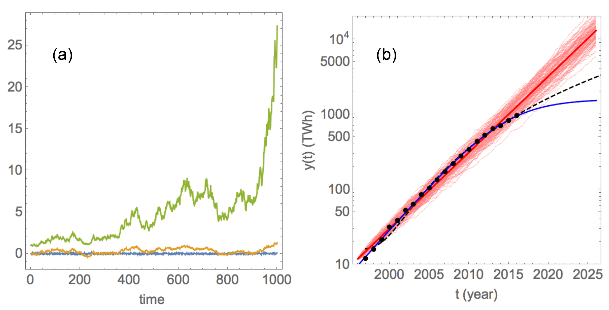
Figure 2 (a) The blue curve is a realisation of a Gaussian white noise process. The yellow curve is a realisation of the random walk given by the cumulative sum of the white noise. The green curve is a realisation of the corresponding geometric Brownian motion with drift coefficient $\mathit{\mu }-{\mathit{\sigma }}^{\mathrm{2}}/\mathrm{2}=\mathrm{0.002}$. (b) The black dots represent the global wind power consumption time series, and the red and blue thick curves represent the linear and log-logistic least-square fit to the logarithm of this time series, respectively. The black, dashed curve is the fit of the power-law model discussed in Sect. 3.2. The thin wiggly, red curves are 100 realisations of the BS process with model parameters that are estimated from the time series data.

2.4 The nature of the noise

From the analysis in the upcoming Sect. 3 (in particular Figs. 3 and 4), we will observe that the residuals obtained from subtracting z(t) from the log-data time series vary relatively smoothly from one year to the next, but sampled on five years intervals they may be consistent with a random walk. For instance, it will be shown that the autocorrelation time is about four years for the residual wind time series. The smooth appearance of the log-residuals on annual scales has important implications for the statistical significance of the downward trend of the relative growth rate claimed by Hansen et al. (2017b). The relative growth rate is defined as the slope of the log-data curve, $y^{\prime }/y=z^{\prime }$, and is constant in time for exponential growth. Hansen et al. (2017b) make a linear regression to the differences $\mathrm{\Delta }{z}_i=z_i-z_{i-\mathrm{1}}$, $n=\mathrm{1},\mathrm{\dots },\mathrm{19}$ and estimate a negative slope of this trend line which is claimed to be significantly different from zero. Such significance estimates, however, are only valid if the noise in Δz_i on annual scale is a Gaussian i.i.d. process. The statistical significance of the negative slope depends critically on the number of independent data points, and if the fluctuations in Δz_i are independent only on time scales longer than four years, there are effectively not more than five such points in the data record, and this is clearly not enough to detect a significant trend in these data.

Figure 3 The black bullets represent global solar power consumption data for the period 1997–2015, and the green bullet for 2016; all according to BP Statistical Review of World Energy (2017). In panel (a), the red and blue curves are exponential and logistic model fits to the 1997–2015 data, respectively. The green, dashed curves are fits to the 1997–2016 data. In the logarithmic plot in panel (b), the blue curve, and the green, dashed curve on top of it (almost invisible) is a fit of the logarithm of the logistic model to the logarithm of the data with the parameter P_max fixed to 550 TWh. For the green curve, the green point is included, for the blue curve, it is not. The other curves are similar fits with P_max fixed to 10³, 10⁴, 10⁵, and 10⁶ TWh, respectively. The residual Q₂ decreases monotonically to the value corresponding to an exponential fit as $P_{max}\to \mathrm{\infty }$.

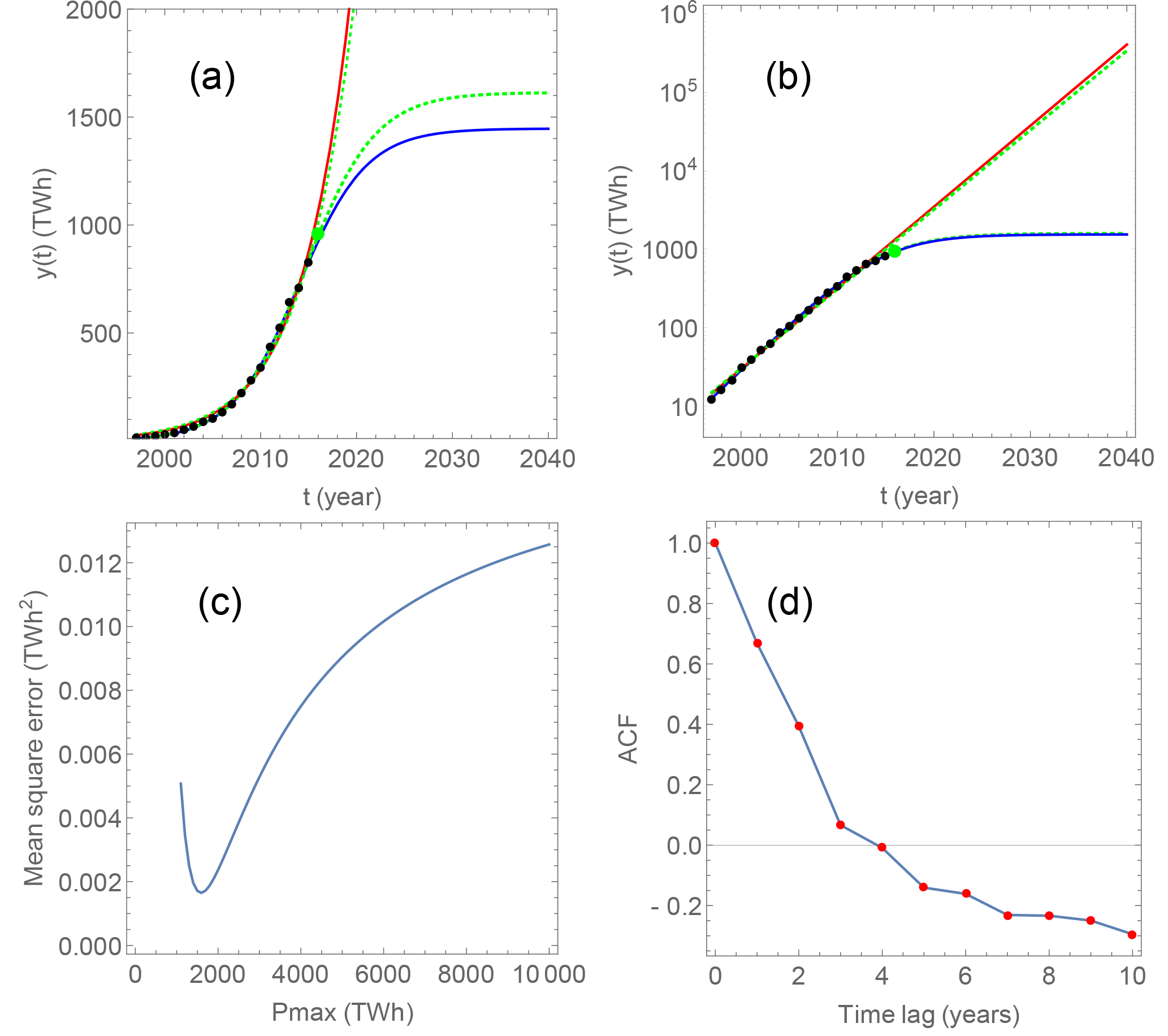
Figure 4 The black bullets represent global wind power consumption data for the period 1997–2015, and the green bullet for 2016; all according to BP Statistical Review of World Energy (2017). In panel (a), the red and blue curves are exponential and logistic model fits to the 1997–2015 data, respectively. The green, dashed curves are fits to the 1997–2016 data. The logarithmic plot in panel (b) shows the fits of the logarithms of these models to the logarithms of the data. Panel (c) shows Q₂ versus P_max, when fitting is made with fixed P_max. The blue curve in panel (b) is the fitted curve with the value of P_max fixed to the minimum of the graph in panel (c). Panel (d) shows the ACF for the residual deviation between the data and the exponential fit.

2.5 Testing the alternative logistic growth hypothesis

The problem we deal with in this paper is to search for evidence for saturation of exponential growth in time series data that to the first order are well described by an exponential function. More precisely, we try to find criteria by which we can reject the BS model (exponential growth) in favour of the SLGM (saturated growth). Hence, in this case it is natural to treat the BS model as the null hypothesis, and the SLGM as the alternative hypothesis. Here, we shall make the test for the wind-power data, since it will be shown in Sect. 3 that the SLGM can be rejected on other grounds for solar power data.

The first step is to perform a least-square fit of the logarithms of the exponential and logistic models to the logarithm of the data.¹ The exponential fit appears as a straight line in the log-log plot, and the sigmoid logistic curve starts out as a straight line with slope μ, gradually bending over to a straight line with zero slope as the growth saturates. The exponential model contains two model parameters y₀ and μ, while the logistic model contains three; y_m, μ, and t_s, and we note that the exponential model is a special case of he logistic since the latter reduces to the exponential in the limit $\mathit{\mu }(t_{\mathrm{s}}-t)\gg \mathrm{1}$. Hence, the logistic model should provide a better fit than the exponential to any data set in terms of the standard deviation of the residual $\sqrt{Q_{\mathrm{2}}}$ given by Eq. (2).

The parameter estimation described above is associated with statistical uncertainty, which will be provided by standard fitting routines as the “standard error” of the estimation. This is presumably what is done to obtain the confidence intervals on the logistic fit in Fig. 3 of Hansen et al. (2017b). These error estimates are based on the assumption that the observed data can be modelled by Eq. (1), where f(t;α) is either the exponential or the logistic function, α the corresponding model parameters, and ϵ(t) a Gaussian white noise process. As explained in Sect. 2.2, it is generally recognised, however, that variables describing the volume of an expanding market is much more adequately described by models of the type Eqs. (3) or (6). This means that the estimation of the model errors (the uncertainty in the model coefficients) must be based on those stochastic models.

Since the question is whether or not we can reject the BS model (the null hypothesis) from the data we explore the implications of that model. It is important to keep in mind that when testing a null hypothesis one has to assume that all assumptions of that hypothesis are true when we explore the implications of the hypothesis, even if one does not believe that they are true. For instance, according to Eq. (3) the residual obtained by subtracting the fitted z(t) from the log-data should be modelled as a Wiener process. To make sure that the downward curving indicated by the three last data points does not contribute to the estimate of the mean and variance of this Wiener process, these points are dropped before estimating the process parameters. After estimating the mean and variance of this process from the residual data,² one can produce an ensemble of numerical realisations of the processes described by Eq. (3). Such an ensemble of realisations is shown for wind power as the cloud of thin wiggly curves in Fig. 2b. The extent of this cloud indicates the uncertainty of the realisations of the fitted model. We could have used this cloud to compute 95 % confidence intervals, but this cloud of 100 realisations actually illustrates better that the observed time series (the black dots) is a possible realisation of the BS model and hence consistent with exponential growth. The blue curve is the fit of the logistic model, and is a clearly better fit in terms of Q₂, but that is obvious due to the additional freedom arising from an additional model parameter.

3 Results for solar and wind power consumption

3.1 Exponential versus logistic growth

The blue and red curves in Fig. 3a show the exponential and logistic least square fits to the time series of global solar power consumption for the period 1997–2015, and the green dotted curves show the effect of including the data point for 2016 (the green dot). It illustrates that by fitting an exponential model to the exponentially growing consumption data, the result becomes very sensitive to the last data points, since these are so large compared to the early part of the time record. However, when we attempt to fit the logarithm of the logistic model to the logarithm of these data it turns out that the best fit (least Q₂) is obtained in the exponential limit $P_{max}\to \mathrm{\infty }$, t_p→∞. In order to check this result, the fitting routine has been applied with fixed $P_{max}=\mathrm{550}$, 10³, 10⁴, 10⁵, 10⁶. The results are shown in Fig. 3b as the blue, gray, yellow, green, and red curves, and the corresponding values of the least square deviation are Q₂=0.1608, 0.1411, 0.1230, 0.1214, 0.1212. This means that, even though the logistic model has one more degree of freedom, the exponential model yields a better fit, and it is not possible to estimate a growth limit by fitting the logistic model to the data. In Sect. 3.2 we shall consider another growth model that makes more sense for these and other data.

A similar analysis has been done to wind power consumption data in Fig. 4a and b. For these data, however, a well defined minimum for Q₂ is found for the logarithmic fit and is shown by the blue curve in Fig. 4b. On top of this curve, but barely visible, is a green, dashed curve representing the fit with the last green point of 2016 included. It serves to demonstrate how the sensitivity to the last points in the time series is reduced by fitting logarithms rather than the raw consumption data. Fig. 4c shows Q₂ versus P_max, when fitting is made with fixed P_max. It shows a well defined minimum, which corresponds to the blue curve in Fig. 4b. In Fig. 4d is plotted the autocorrelation function (ACF) for the residual deviation between the data and the exponential fit. It shows an autocorrelation time of around four years, hence the residual for the entire data series contain no more than five data points that can be considered independent.

3.2 Power-law growth – a middle ground

It is clear from Fig. 1a that continuing exponential growth for solar and wind power beyond 2030 implies volumes that seem almost unthinkable. Hence, it is not unreasonable to consider the possibility that the declining relative growth rate $z^{\prime }=y^{\prime }/y$ observed for wind power in Fig. 2b is the manifestation of a declining trend in this growth rate. What is demonstrated in that figure is not that this decline is not real, but that it is not statistically significant for the time series data at hand. But even if we assume that this decline is real, the correct model does not have to be the logistic one. The logistic model requires complete saturation of the growth for times well beyond t_p, while some regional data, for instance wind consumption in Europe, seem to display non-saturating growth slower than exponential. Actually a third-order polynomial can be very accurately fitted to those data. By examining many regional data sets in logarithmic plots there seems to be a curve which is linear (exponential growth), or even curving upwards, up to a certain year, and then a logarithmic-like curve after this year. This is in fact also what we observe in the global solar consumption data.

Suppose we identify a year after which the logarithm of the consumption time record exhibits such a logarithmic growth, and let us drop all data prior to that year. A model that captures this logarithmic behaviour has the form

$$\begin{array}{}\text{(8)}& y\left(t\right)=p(t+t_{\mathrm{0}}{)}^q,\end{array}$$

since it implies that $\ln y\left(t\right)=\ln p+q\ln (t+t_{\mathrm{0}})$. Here the origin of the time axis is chosen at the first year of the new shorter time series and t₀ then is a positive number. The power-law model is a solution of the differential equation

$$\begin{array}{}\text{(9)}& {\displaystyle \frac{\mathrm{d}y}{\mathrm{d}t}}={\displaystyle \frac{q}{t+t_{\mathrm{0}}}}y,\end{array}$$

which is just the equation for exponential growth with a time-dependent relative growth rate $\mathit{\gamma }\left(t\right)=q/(t+t_{\mathrm{0}})$. By adding a multiplicative noise term on the right hand side, Eq. (9) can easily be cast into the form of a generalised BS equation.

When an exponential model was fitted to the data, the idea was to make use of the entire time series and give equal weight to the early and late stages of the growth. This is why it was appropriate to fit the linear model to the logarithm of the data. The power-law model, however, is expected to describe only the latest decade of the historical growth, and the advantage of fitting the logarithm of the power-law model to the logarithm of the data is not so obvious. The two methods give similar results, and those presented in Fig. 1b are for the power-law model fitted to the consumption data without taking logarithms.

For the global solar power consumption, the time series prior to 2007 does not fit to the model and must be discarded. The fit for the period 2008–2016 is shown as the red curve in Fig. 1b. For global wind power consumption, the entire time series can be used meaningfully, but the last decade is expected to contain more relevant information about the time-dependent growth rate. The latter yields a slightly lower q and the fit is shown as the blue curve in Fig. 1b. The residual variances Q₂ are considerably lower than the corresponding for the fitted exponential model (the fit is much better), but this is expected since the number of model parameters is three for the power law model and two for the exponential model.

The estimated growth exponents are q≈2.7 for solar power and q≈2.0 for wind power. This implies that the solar power consumption overtakes wind power around 2034, a few years later than predicted by the exponential growth model. According to the REmap scenario this would happen just after mid-century.

For the power-law model the underlying assumption is that it is not a good model up to certain date, where constraining factors start to kick in. That date can only be established by examination of the data. For wind power the result is quite insensitive to the choice of this date, but the fit is best if I choose it as late as 2007. For solar power the growth is faster than exponential before 2007, and the best fit is found if 2008 is chosen as a start date. That gives 10 data points to fit for wind and 9 data points for solar. Choosing a later start date has negligible effect on the fitted curves. Hence the results of the fitting procedure is quite robust as long as the start date is chosen after the saturation of the exponential growth has become visible in the data, i.e. after the slope of the logarithmic plot has started to decrease.

It should be emphasised that this is not cherry-picking, but construction of a model that has a limited range of validity and based on the available data. It is also important to keep in mind that there is also an upper time limit for the validity of the power-law model, since it exhibits unlimited growth as t goes to infinity. In this paper I have assumed that it holds at least up to 2050, but sooner or later the actual growth will have to stall due to planetary boundaries.

3.3 Why power-law growth?

In this subsection it is shown that power-law growth plays a particular role in the class of growth models with relative growth rates γ(t) that decay towards zero as t→∞. A general growth model for the variable y(t) is one where we have a time-dependent relative growth rate γ(t), i.e. we have the differential equation

$$\begin{array}{}\text{(10)}& {\displaystyle \frac{\mathrm{d}y}{\mathrm{d}t}}=\mathit{\gamma }\left(t\right)y,\end{array}$$

with the solution

$$\begin{array}{}\text{(11)}& y=y\left(\mathrm{0}\right)\exp \left[\underset{\mathrm{0}}{\overset{t}{\int }}\mathit{\gamma }\right(t^{\prime }\left)\mathrm{d}{t}^{\prime }\right].\end{array}$$

Note that the growth saturates to a finite value only if the integral ${\int }_{\mathrm{0}}^{\mathrm{\infty }}\mathit{\gamma }\left(t^{\prime }\right)\mathrm{d}{t}^{\prime }$ is finite. Let us now consider a wider class of relative growth rates than considered in Section 3.2, namely those that decay algebraically towards zero as t→∞ with an arbitrary positive exponent μ;

$$\begin{array}{}\text{(12)}& \mathit{\gamma }\left(t\right)={\displaystyle \frac{q}{(t+t_{\mathrm{0}}{)}^{\mathit{\mu }}}},t_{\mathrm{0}}\ge \mathrm{0},\mathit{\mu }\ge \mathrm{0}.\end{array}$$

The case μ=1 yields the power-law growth

$$\begin{array}{}\text{(13)}& y\left(t\right)={\displaystyle \frac{y\left(\mathrm{0}\right)}{t_{\mathrm{0}}^q}}(t+t_{\mathrm{0}}{)}^q\end{array}$$

which was treated in Sect. 3.2. For μ≠1 the general solution is

$$\begin{array}{}\text{(14)}& y\left(t\right)=y\left(\mathrm{0}\right)\exp \left[{\displaystyle \frac{q}{\mathrm{1}-\mathit{\mu }}}\left((t+t_{\mathrm{0}}{)}^{\mathrm{1}-\mathit{\mu }}-t_{\mathrm{0}}^{\mathrm{1}-\mathit{\mu }}\right)\right].\end{array}$$

Hence, for μ<1 we have unlimited growth which for t→∞ has the asymptotic form

$$\begin{array}{}\text{(15)}& y\left(t\right)=y\left(\mathrm{0}\right)\exp \left[{\displaystyle \frac{q}{\mathrm{1}-\mathit{\mu }}}{t}^{\mathrm{1}-\mathit{\mu }}\right],\end{array}$$

which means faster-than-exponential growth for μ<0, exponential growth for μ=0, and slower-than-exponential growth for $\mathrm{0}<\mathit{\mu }<\mathrm{1}$. For μ>1 it is convenient to rewrite Eq. (14) in the form

$$\begin{array}{}\text{(16)}& y\left(t\right)=y\left(\mathrm{0}\right)\exp \left[{\displaystyle \frac{q}{\mathit{\mu }-\mathrm{1}}}\left({\displaystyle \frac{\mathrm{1}}{t_{\mathrm{0}}^{\mathit{\mu }-\mathrm{1}}}}-{\displaystyle \frac{\mathrm{1}}{(t+t_{\mathrm{0}}{)}^{\mathit{\mu }-\mathrm{1}}}}\right)\right].\end{array}$$

The growth in this case is limited, and the solution increases monotonically towards the limit

$$\begin{array}{}\text{(17)}& y\left(t\right)=y\left(\mathrm{0}\right)\exp \left[{\displaystyle \frac{q{t}_{\mathrm{0}}^{\mathrm{1}-\mathit{\mu }}}{\mathit{\mu }-\mathrm{1}}}\right].\end{array}$$

The power-law growth for μ=1 is thus neatly poised between the slower-than-exponential growth of Eq. (15) for $\mathit{\mu }\to {\mathrm{1}}^{-}$ and the limited growth of Eq. (16) for $\mathit{\mu }\to {\mathrm{1}}^{+}$. It is thus a natural model for growth that slows down with time, but for which the growth is not yet determined by a definite growth limit set by physical boundaries.

4 Discussion

The renewable energy sector is an integrated part of the global economy that grows in importance at the expense of fossil-fuel based energy production and consumption. Its growth is essentially governed by the same laws that govern other sectors of the economy. Sectors grow at different rates, depending on complex market mechanisms, economic policy strategies by governments and international bodies, and in some cases by boundaries set by the availability of natural resources and land. The effect of scarcity of resources is definitely felt in the fossil fuel sector. However, the decline, and eventually negative sign, of growth in this sector will not be determined by the physical limit of exploitable resources. The decline will be determined by the competition with the non-fossil energy sectors, by the pace of technological advances in those sectors, and by how well the international community will succeed on implementing carbon pricing reflecting the actual social cost of carbon.

The two IEA and IRENA scenarios used in this paper are the results of macroeconomic modeling based on assumptions of rapid technological progress in the renewable energy sector, of successful implementation of climate mitigation policies, and absence of definite limits set by scarcity of resources and land. Neither of these assumptions can be proven at present. For instance, the physical availability of unexploited land up to 2050 is unquestionable, but there is already strong public opposition against vast wind farms and solar power installations in many countries. It is impossible to predict or model the outcome of the political battles over such issues, hence any attempt to justify a simple dynamical model by suggesting specific constraining mechanisms will appear as arbitrary and ad hoc. This is why this paper has a focus on the construction of simple empirical rather than dynamical models.

Thus, in this paper, no attempts have been made to derive the three statistical models under consideration from physical and/or economic laws. That does not mean that they cannot be interpreted in the light of such laws. The exponential growth law that underpins the BS-equation is based on the assumption that the capital available to expand production at a given time is proportional to the production volume at this time. This implies that the relative growth rate $\mathit{\gamma }\left(t\right)=y^{\prime }/y$ is independent of time. Since the logistic growth law assumes that $\mathit{\gamma }\left(t\right)=\mathit{\mu }[\mathrm{1}-y(t)/y_m]$, it implies that the relative growth rate goes to zero as the volume y reaches a certain limit y_m. This typically models a situation where the growth rate depends on a resource that is depleted as the volume grows. For solar and wind power this could be the availability of suitable land areas, crucial raw materials, or investment capital.

On the other hand, for renewable power there is no good reason why the growth rate should go to zero at a particular volume of production, and the macroeconomic modelling underlying the scenarios of IEA and IRENA does not support that such a limit will be attained during the first half of this century. The power-law model was found to give very good fits to the data throughout the last decade. One cannot conclude that this model is preferable based on the historical data only, but the predictions are close to the 2^∘ scenarios of IEA and IRENA, while those of the exponential and the logistic models are way off.

5 Conclusions

The paper has examined three empirical growth models whose parameters are determined by fitting to historical data for solar and wind power consumption. According to the principle of parsimony the simplest model consistent with the data is preferable, and in our study this is the exponential model, since it contains only two model parameters. The snag here, of course, is that the two more complex models yield better fit to the data, and hence it does not seem possible to select the best model from such principles.

It is clear from Fig. 2b that the exponential model is not rejected by the data, and it cannot be excluded that the near future will unfold as a realisation of a geometric brownian motion, i.e. as an exponential growth with multiplicative noise. In that case, the declining relative growth rate during the last five years should be interpreted as a market fluctuation. On the other hand, one cannot rule out that the decline of the growth rate is the start of a continuing trend. One model to describe such a trend is the logistic model, which describes a rapid convergence to a zero growth rate. For solar power data it is not possible to estimate the parameters of the logistic model, i.e. the optimal logistic model is reduced to the exponential. For wind power consumption the predicted limit is less than 50 % above the present level, which is only half of the wind consumption in the pessimistic IEA current policies scenario and one fourth of the prediction in the 450 scenario (IEA, 2016). Thus, the predicted limit of the logistic model seems unrealistically low, and hence casts doubt about the relevance of this growth model.

On the other hand, the $\mathit{\gamma }\left(t\right)\propto \mathrm{1}/t$ time dependence of the power-law model is what yields good fit to the historical data as well as to the 2^∘ target scenario of IEA and IRENA. In fact, this match to historical and scenario data suggests a remarkable simple empirical law: the relative growth rate of renewable energy consumption decays inversely proportional to time. In Sec. 3.3 it was shown that that this growth law appears as a special case of a wider class of growth models for which the relative growth rate $\mathit{\gamma }\left(t\right)=y^{\prime }/y$ decays algebraically towards zero, i.e. as $\mathit{\gamma }\left(t\right)\sim (t+t_{\mathrm{0}}{)}^{-\mathit{\mu }}$. This special case (μ=1) constitutes the borderline between slower than potential unlimited growth (μ<1) and limited growth (μ>1).

The years to come will show if the data points will continue to fall on the power-law trajectories of Fig. 1b. If they do, they will begin falling outside the confidence cloud of Fig. 2b around 2020 and thus reject the exponential growth hypothesis. Thus, after this date we may be able to make a more educated selection among models for predicting the growth of these renewable energies through the first half of this century.