Verification of TRANSPORT Simulation Environment coupling with PHREEQC for reactive transport modelling

Many types of geologic subsurface utilisation are associated with fluid and heat flow as well as simultaneously occurring chemical reactions. For that reason, reactive transport models are required to understand and reproduce the governing processes. In this regard, reactive transport codes must be highly flexible to cover a wide range of applications, while being applicable by users without extensive programming skills at the same time. In this context, we present an extension of the Open Source and Open Access TRANSPORT Simulation Environment, which has been coupled with the geochemical reaction module PHREEQC, and thus provides multiple new features that make it applicable to complex reactive transport problems in various geoscientific fields. Code readability is ensured by the applied high-level programming language Python which is relatively easy to learn compared to low-level programming languages such as C, C++ and FORTRAN. Thus, also users with limited software development knowledge can benefit from the presented simulation environment due to the low entry-level programming skill requirements. In the present study, common geochemical benchmarks are used to verify the numerical code implementation. Currently, the coupled simulator can be used to investigate 3D single-phase fluid and heat flow as well as multicomponent solute transport in porous media. In addition to that, a wide range of equilibrium and nonequilibrium reactions can be considered. Chemical feedback on fluid flow is provided by adapting porosity and permeability of the porous media as well as fluid properties. Thereby, users are in full control of the underlying functions in terms of fluid and rock equations of state, coupled geochemical modules used for reactive transport, dynamic boundary conditions and mass balance calculations. Both, the solution of the system of partial differential equations and the PHREEQC module, can be easily parallelised to increase computational efficiency. The benchmarks used in the present study include density-driven flow as well as advective, diffusive and dispersive reactive transport of solutes. Furthermore, porosity and permeability changes caused by kinetically controlled dissolution-precipitation reactions are considered to verify the main features of our reactive transport code. In future, the code implementation can be used to quantify processes encountered in different types of subsurface utilisation, such as water resource management as well as geothermal energy production, as well as geological energy, CO₂ and nuclear waste storage.

1 Introduction

Geologic subsurface utilisation requires tools for quantitative and predictive assessments to mitigate potential risks for health and the environment as well as to increase the overall efficiency by iterative process optimisation. In this context, the numerical simulation of coupled processes provides insights for stakeholders, operators, governmental authorities and decision makers for many decades. Here, especially the flexibility of the applied simulation tools in view of their extendability and adaptability to specific scientific questions and technical challenges is of critical importance. Example applications which require the flexibility to undertake modifications of existing numerical codes include the formation of gas hydrates and permafrost at laboratory to field scales, e.g., (Li et al., 2022a, b) as well as dissolution processes in potash seams, e.g., Steding et al. (2021a, b) among others. Many commercially available but also scientific numerical simulation tools do not offer the required flexibility to couple arbitrary chemical modules to fluid flow and species transport, or are often limited by the requirement of learning a low-level programming language such as FORTRAN, C or C++, etc. to allow for the required adaptations.

For that reason, Kempka (2020) implemented a TRANSPORT Simulation Environment (TRANSPORTSE) to simulate density-driven fluid flow, advective, diffusive and dispersive species as well as conductive and convective heat transport. TRANSPORTSE is written in the easy-to-learn Python programming language (Van Rossum and Drake, 2009) and is flexible in terms of the integration of third-party libraries and modules, including fluid and rock equations of state, e.g., CoolProp (Bell et al., 2014), chemical reaction models, e.g., Cantera (Goodwin et al., 2017), and hydrogeochemical reaction models, e.g., PHREEQC (Parkhurst and Appelo, 2013). The present contribution demonstrates the feasibility of the proposed concept based on the coupling of TRANSPORTSE with the widely-applied geochemical reaction module PHREEQC (Parkhurst and Appelo, 2013). For that purpose, a series of numerical simulation benchmarks derived from Engesgaard and Kipp (1992) as well as Poonoosamy et al. (2021) are used to verify the hydrogeochemical process coupling implementation, referred to as TRANSPORTSE-PHREEQC in the following.

2 Materials and Methods

In the next subsections, the coupling between the TRANSPORTSE and PHREEQC software packages as well as the five applied numerical benchmark studies are briefly introduced.

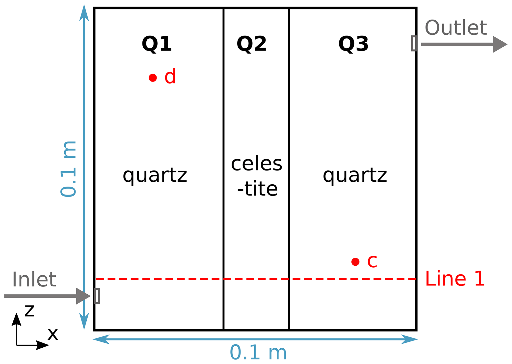
Figure 1 Poonoosamy et al. (2021) benchmark model geometry with location of observation points (c) and (d) as well as Line 1. The initial solution is injected at the inlet, flowing through regions of three different mineralogies (Q1, Q2 and Q3), with the resulting solution leaving the flow cell via the outlet.

2.1 TRANSPORT Simulation Environment (TRANSPORTSE) and PHREEQC

The TRANSPORT Simulation Environment (TRANSPORTSE) makes use of the Finite Difference Method to solve the density-driven formulation of the Darcy flow equation, coupled with the equations for transport of heat and chemical species on structured grids by simple explicit, weighted semi-implicit or fully-implicit numerical schemes. Just-in-time compilation is implemented using the Python Numba library (Lam et al., 2015) and results in a computational efficiency in the same order of equivalent low-level language implementations (e.g., FORTRAN, C or C++). Further, CPU-based parallelisation (Anderson et al., 2017) enables high spatial model discretisations (Kempka, 2020). TRANSPORTSE uses a modular Python configuration file which allows the user to write individual functions for fluid and rock properties as well as chemical reactions, which are then sequentially called during the code execution. Furthermore, functions can be defined to, e.g., dynamically assign time-dependent model boundary conditions and calculate arbitrary mass balances. The use of the Python language provides the user with full read and write access to any model parameter that may be of relevance to answer a specific scientific question.

The coupling of PHREEQC is realised by means of the phreeqpy software package (Charlton and Parkhurst, 2011), which acts as a Python interface to the IPhreeqc module. The phreeqpy library is initiated via the aforementioned configuration file, and the user has all flexibility to dynamically define the required IPhreeqc input data with the help of the TRANSPORTSE function dedicated to chemical reactions. As chemical reaction modelling is almost always the computational bottleneck in reactive transport simulations, TRANSPORTSE allows for a CPU-based parallelisation of the chemical module runs, so that coupled hydrochemical models with relatively high spatial discretisations become computationally feasible. Chemical surrogate models may be also easily integrated with TRANSPORTSE if the computational demand of the chemical models can be reduced by their implementation without a significant loss in accuracy.

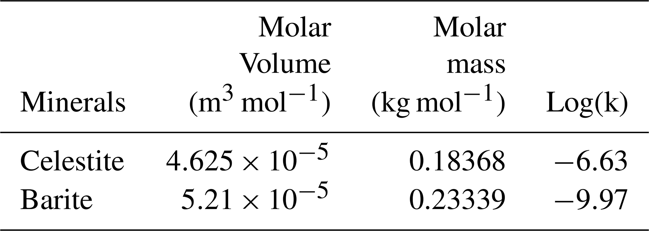
Table 1 Applied mineral properties based on PHREEQC phreeqc.dat database and Poonoosamy et al. (2021).

2.2 Hydrogeochemical Simulation Benchmarks

Two different chemical systems with a step-wise increase in complexity have been used for the verification of the TRANSPORTSE-PHREEQC implementation. The first benchmark is a relatively simple 1D advective transport model with chemical reactions (Engesgaard and Kipp, 1992), whereby the TRANSPORTSE-PHREEQC implementation is tested against an implementation solely based on PHREEQC. Further, the second benchmark employs a 2D model and adds different processes, such as density-driven flow, reactive surface area changes as well as porosity and permeability changes (Poonoosamy et al., 2021). TRANSPORTSE-PHREEQC simulation results are compared with those produced by five established reactive transport codes, including CORE2D (Samper et al., 2009), MIN3P-THCm (Mayer et al., 2002), OpenGeoSys-GEM (Kosakowski and Watanabe, 2014), PFLOTRAN (Lichtner et al., 2017) and TOUGHREACT (Xu et al., 2011).

2.2.1 Engesgaard and Kipp (1992) Benchmark

The computationally challenging benchmark introduced by Engesgaard and Kipp (1992) and applied by many different authors, e.g., Shao et al. (2009), Leal et al. (2020), and De Lucia and Kühn (2021a, b), is used in the present study to verify the coupling between purely advective species transport (TRANSPORTSE) and chemical reactions (PHREEQC). The hereto applied 1D model consists of 50 elements, whereby a total model length of 1 m is assumed. A Neumann flow boundary condition is applied at the left boundary (x=0 m) and the solution is shifted by PHREEQC by one element every 999 s until a total amount of 30 shifts is achieved. The porosity amounts to 32 %, and diffusion, dispersion and density-driven flow are neglected in this benchmark.

With regard to hydrochemistry, the initial solution is saturated with calcite (CaCO₃) and exhibits a pH = 9.91 at a reference temperature of 25 ^∘C. A MgCl₂ solution enters the model at the left boundary with a concentration of 0.001 mol kgw⁻¹. Hereby, dolomite is formed by Reaction 1, while dissolution and precipitation processes are determined by reaction kinetics, resulting in pH and density changes of the solution.

$$\begin{array}{}\text{(1)}& \mathrm{2}{\mathrm{CaCO}}_{\mathrm{3}}+{\mathrm{MgCl}}_{\mathrm{2}}\to \mathrm{CaMg}({\mathrm{CO}}_{\mathrm{3}}{)}_{\mathrm{2}}+{\mathrm{CaCl}}_{\mathrm{2}}\end{array}$$

To test the correct implementation of chemical reactions via the chemical reaction function in the TRANSPORTSE configuration file, the spatial distribution of mineral and species concentrations as well as pH along the 1D model dimension at the end of the simulation time are compared against the reference.

2.2.2 Poonoosamy et al. (2021) Benchmarks

The second benchmark is composed of four different sub-benchmarks in total, whereof three are considered in the present study. Hereby, the complexity of the coupled hydrochemical model is increased with each sub-benchmark. Figure 1 shows the 2D flow cell experiment executed by Poonoosamy et al. (2021) with a spatial extent of 0.1 m × 0.1 m × 0.01 m. The spatial model discretisation uses grid dimensions of 1 mm × 1 mm, resulting in 10 000 elements. The inlet and outlet boundary conditions are distributed along three elements each, with point-symmetric z-coordinates that were chosen to be as close as possible to the coordinates given in Poonoosamy et al. (2021, Table 2). Consequently, the z-coordinates of the inlet are 0.008–0.011 m and those of the outlet 0.089–0.092 m. This results in a source and sink length of 0.003 m instead of 0.0033 m as documented in the source document.

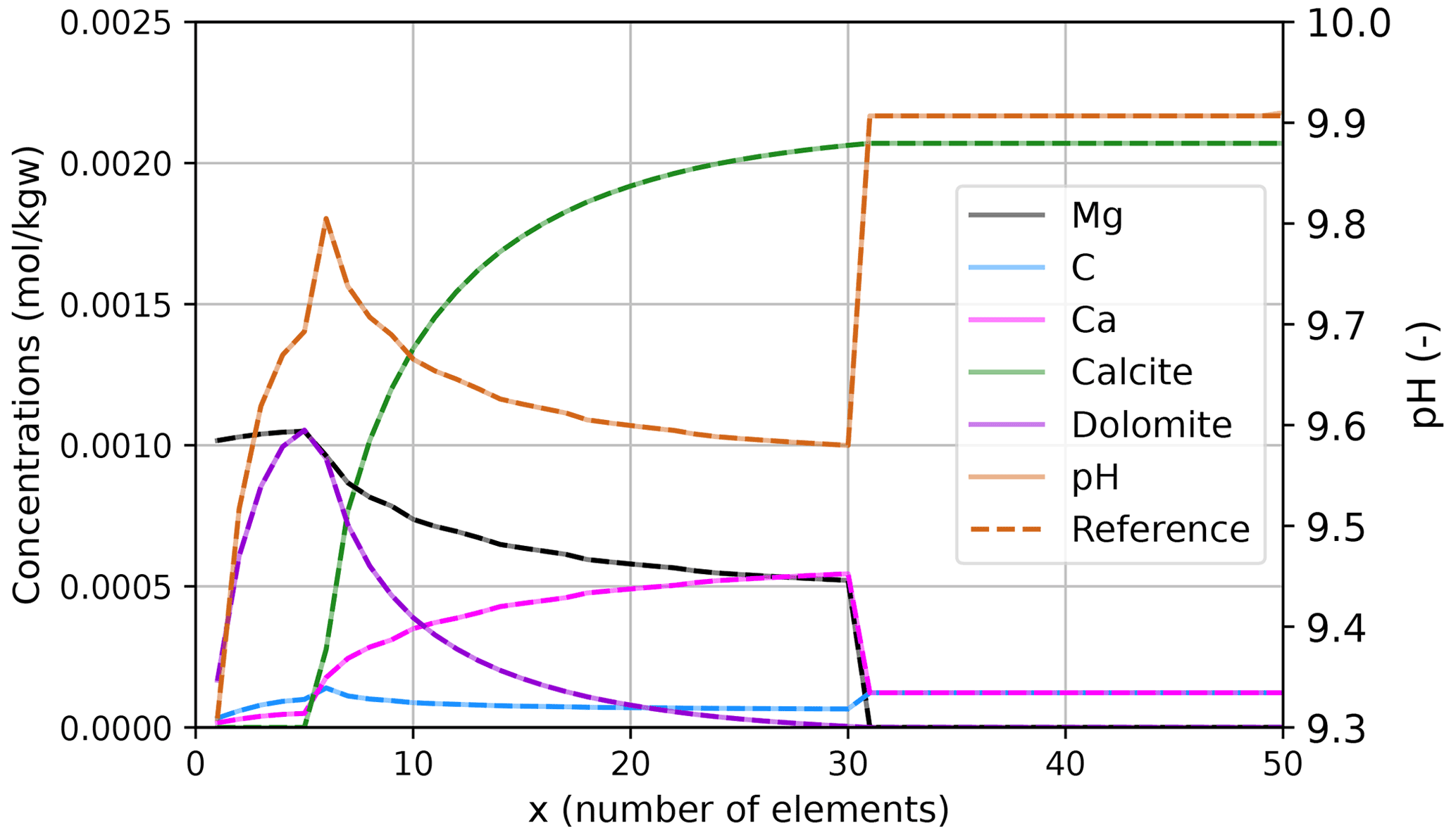
Figure 2 Concentration, pH and mineral profiles comparing the TRANSPORTSE-PHREEQC simulation results against the reference 1D transport model introduced by Engesgaard and Kipp (1992), where a MgCl₂ solution enters the model via the left boundary, with mineral dissolution and precipitation being controlled by reaction kinetics.

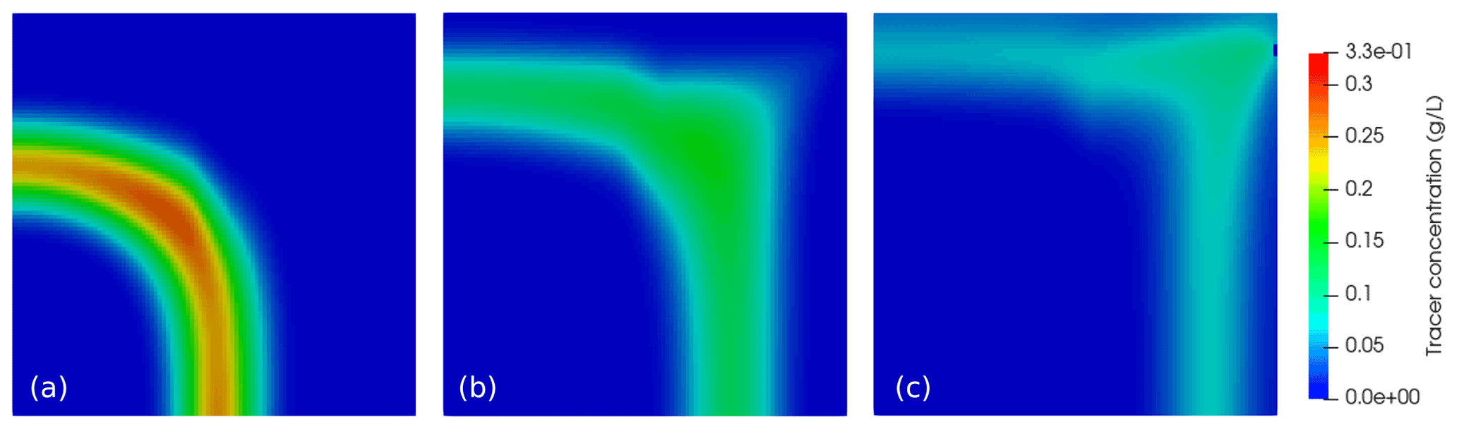
Figure 3 Spatial distribution of tracer concentration calculated with TRANSPORTSE-PHREEQC for simulation times (a) 8 h, (b) 16 h, and (c) 24 h for Case 1 using the same scale mapping as in Poonoosamy et al. (2021, Fig. 3).

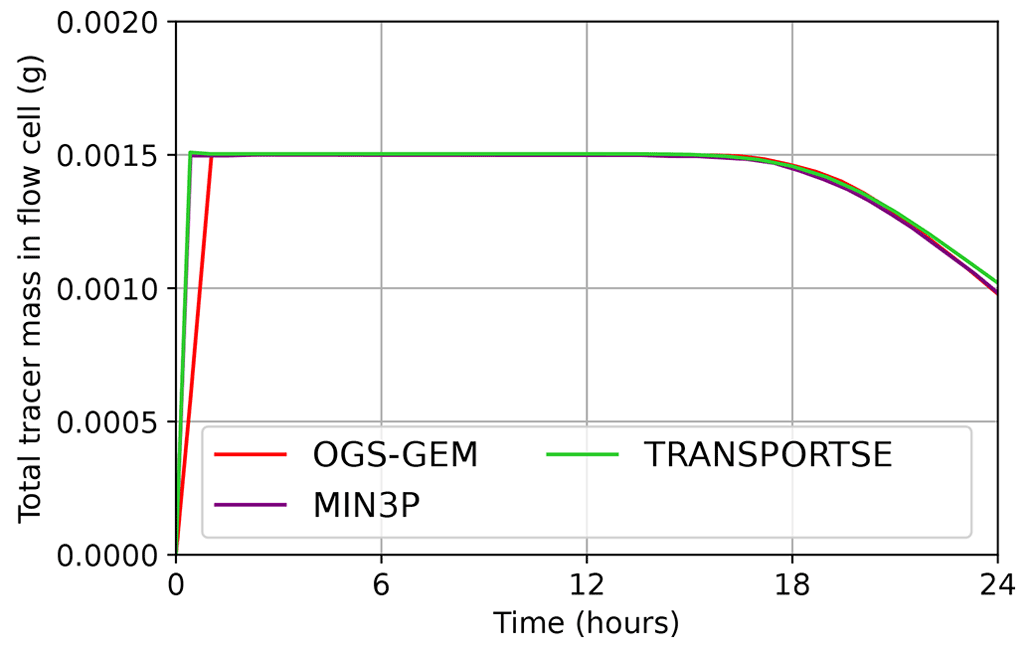
Figure 4 Temporal development of total tracer mass in flow cell calculated by TRANSPORTSE-PHREEQC in comparison against the results produced by MIN3P-THCm and OpenGeoSys-GEM (Poonoosamy et al., 2021).

The fluid inlet is located at the lower left corner, while the outlet is at the upper right, which results in an asymmetric flow field in the flow cell. Two observation points (c) and (d), are located at (x, z) = (0.08, 0.02 m) and (x, z) = (0.02, 0.08 m), respectively. Further, an observation line (Line 1) located at z=0.01 m is used in the result analysis. The model contains three regions of different mineralogy, where Q1 and Q3 contain quartz, while Q2 is filled with celestite.

Dirichlet boundary conditions are applied for the species concentrations at the inlet and outlet elements, whereby a source term with a strength of 20 µL min⁻¹ is used at the inlet and a constant pressure (p=101 325 Pa) at the outlet. Application of dynamic boundary conditions allows to reset the tracer concentration after the specified simulation time. Temperature is assumed to be 25 ^∘C to match with the standard PHREEQC chemical database (phreeqc.dat). Rock density is determined from molar volume and molar mass given in Table 1.

Dynamic viscosity which is not provided by Poonoosamy et al. (2021) is set to 8.9 × 10⁻⁴ Pa s corresponding to that of water at 101 325 Pa and 25 ^∘C. Fluid and rock compressibilities of 4.4 × 10⁻⁹ and 4.5 × 10⁻¹⁰ Pa⁻¹ were assumed due to the lack of information in the source publication, respectively.

The three cases differ in their complexity, whereby Case 1 does consider advective, diffusive and dispersive transport without any chemical reactions. All parameters are chosen according to Poonoosamy et al. (2021, Table 1) with water being injected with the addition of a tracer at a concentration of 3 g L⁻¹ for the first 25 min and no tracer thereafter. Consequently, a total tracer amount of 1.5 mg is injected into the flow cell.

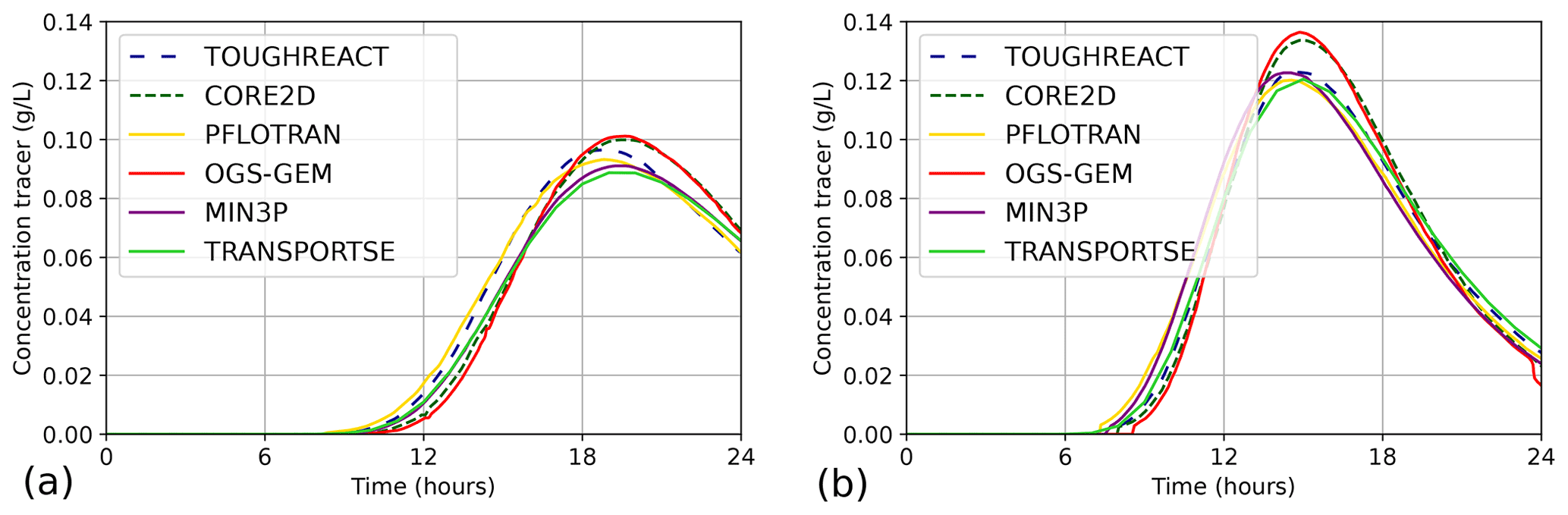
Figure 5 Concentration of tracer at (a) observation points c and (b) d at different times calculated by TRANSPORTSE-PHREEQC in comparison against the results documented by Poonoosamy et al. (2021).

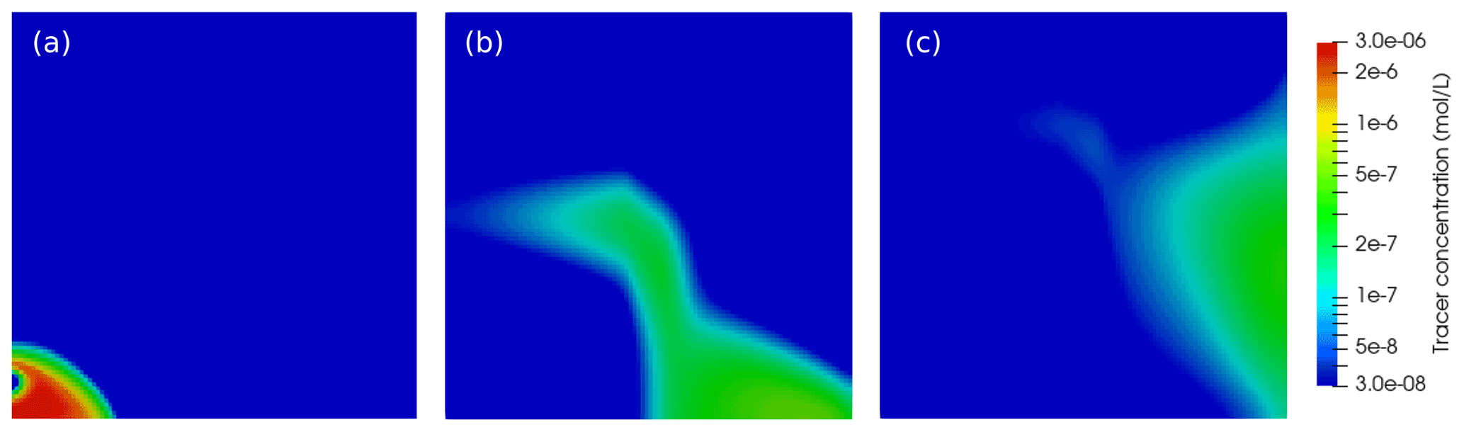
Figure 6 Spatial distribution of tracer concentration calculated with TRANSPORTSE-PHREEQC for simulation times (a) 30 min, (b) 8 h, and (c) 16 h for Case 2 using the same log-scale mapping as in Poonoosamy et al. (2021, Fig. 8).

Case 2 considers density-driven flow, with an initial linear increase in pressure in z-direction is assumed with 101 325 Pa at the model top and a fluid density of 997.04 kg m⁻³, which was calculated with PHREEQC for pure water at a temperature of 25 ^∘C. The tracer concentration at the inlet is set to 3 × 10⁻⁶ mol L⁻¹ for the first 25 min of the simulation and then reset. The concentration of the second species at the inlet (NaCl) is 1.4 mol L⁻¹ and fluid density of the resulting solution 1052.3 kg m⁻³, calculated with PHREEQC. During the simulation, the density from the last time step is used as input for the chemical calculations with the current species concentrations to determine the new density. This is done by an iterative approach with a tolerance of 0.001 kg m⁻³, before the result is used as new density for the following calculations. The increase in solution volume is neglected as the change in water volume is not relevant in the present sub-benchmark.

In Case 3a, mineral dissolution and precipitation result in porosity and permeability changes. Density-driven flow is neglected following Poonoosamy et al. (2021), while density changes are considered for the chemical calculations, since the concentrations calculated by PHREEQC would be wrong otherwise. Here, a BaCl₂ solution is injected at a concentration of 0.3 mol L⁻¹ with a fluid density of 1051.41 kg m⁻³ at the inlet, derived from a PHREEQC pre-calculation. Reaction (R1) induces celestite dissolution and barite precipitation. Only four major species ($\mathrm{Ba},{\mathrm{SO}}_{\mathrm{4}},\mathrm{Sr},\mathrm{Cl}$) and two minerals (barite and celestite) are relevant to Reaction (R1), so that all other components listed in Poonoosamy et al. (2021, Table 5) are neglected. Rock densities of celestite and barite are calculated from the molar volumes listed in the source publication, with an initial amount of celestite of 1.44865 × 10⁻⁴ mol element⁻¹ in Q2, which is slightly different to that used in the source publication. The initial solution in Q2 is saturated with respect to SrSO₄ (celestite) with concentrations of 6.18638 × 10⁻⁴ mol L⁻¹ for Sr²⁺ and ${\mathrm{SO}}_{\mathrm{4}}^{\mathrm{2}-}$ calculated by PHREEQC and a fluid density of 997.15743 kg m⁻³. The decimal place accuracy given here is required for reproducibility.

With regard to the dissolution kinetics of celestite, its initial amount of 1.44397 × 10⁻⁴ mol element⁻¹ consists to one third of small grains (celestite 1) with a large reactive surface area of 20 000 m² m⁻³ and to two thirds of large grains (celestite 2) with a small reactive surface area of 100 m² m⁻³. Here, the volume fraction of both minerals must be known in each model element at any simulation time to derive the total reactive surface area, and thus the amount of dissolved celestite. The initial surface area is A = (0.223 × 20 000 + 0.447 × 100) m² m⁻³, whereby the dissolved amount of celestite is calculated by the rate law given in Eq. (1) with log(k) = −5.66 (reaction constant at 25 ^∘C) and Ω in saturation with respect to celestite.

$$\begin{array}{}\text{(R1)}& {\mathrm{Ba}}^{\mathrm{2}+}+{\mathrm{SrSO}}_{\mathrm{4}}\to {\mathrm{BaSO}}_{\mathrm{4}}+{\mathrm{Sr}}^{\mathrm{2}+}\end{array}$$

$$\begin{array}{}\text{(1)}& {\displaystyle \frac{\mathrm{d}m}{\mathrm{d}t}}=-A\times k\times (\mathrm{1}-\mathrm{\Omega })\end{array}$$

Based on the fraction of each mineral on the total reactive surface, the contribution of each mineral to the total dissolved amount is determined. Consequently, the new mineral amounts and their volume fractions are calculated, so that the new surface area can be determined in the next step. Precipitation kinetics of barite are not considered in the source publication. Hence, thermodynamic equilibrium is assumed to generate its immediate precipitation in case of supersaturation. Porosity is calculated from the present mineral volumes using their densities determined as discussed above. Permeability changes are calculated using the modified Kozeny–Carman equation (Eq. 2) with ϕ₀ and k₀ as initial porosity and permeability, respectively, whereas ϕ and k represent their current values. The water amount in each element is calculated from the fluid density and pore volume and needs to be adapted if porosity changes occur. The input fluid density for the PHREEQC calculations is not iteratively adapted, since the changes are relatively small within one chemical time step. The total simulation time amounts to 300 h.

$$\begin{array}{}\text{(2)}& k=k_{\mathrm{0}}\times {\left({\displaystyle \frac{\mathit{\varphi }}{{\mathit{\varphi }}_{\mathrm{0}}}}\right)}^{\mathrm{3}}\end{array}$$

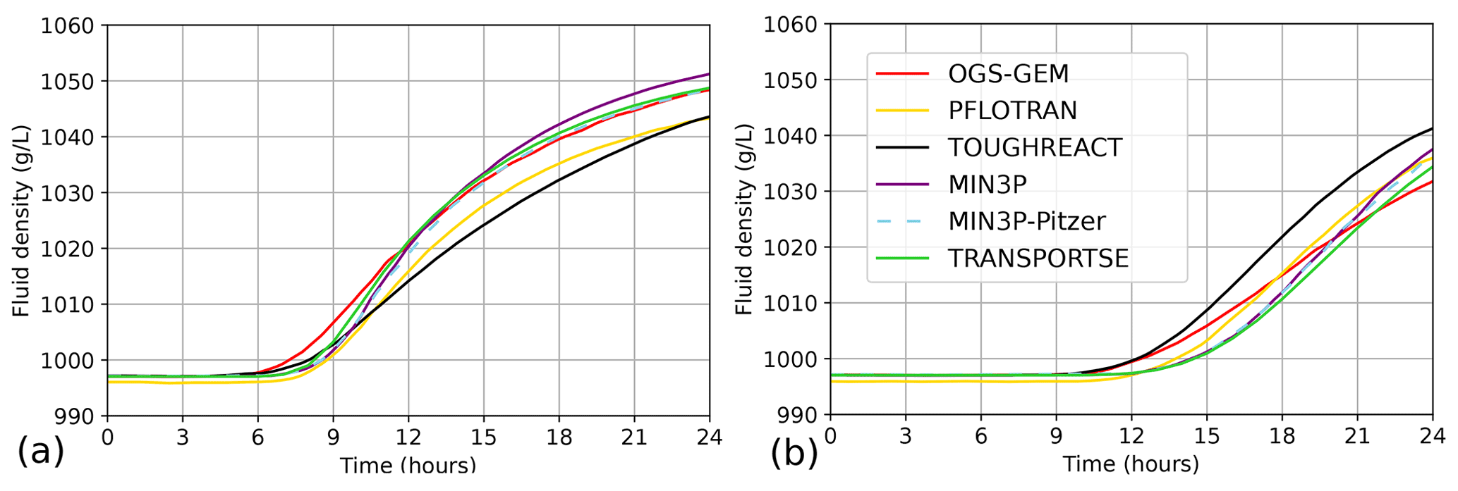
Figure 7 Fluid densities at observation points (a) c and (b) d at different times calculated by TRANSPORTSE-PHREEQC in comparison against the results documented by Poonoosamy et al. (2021).

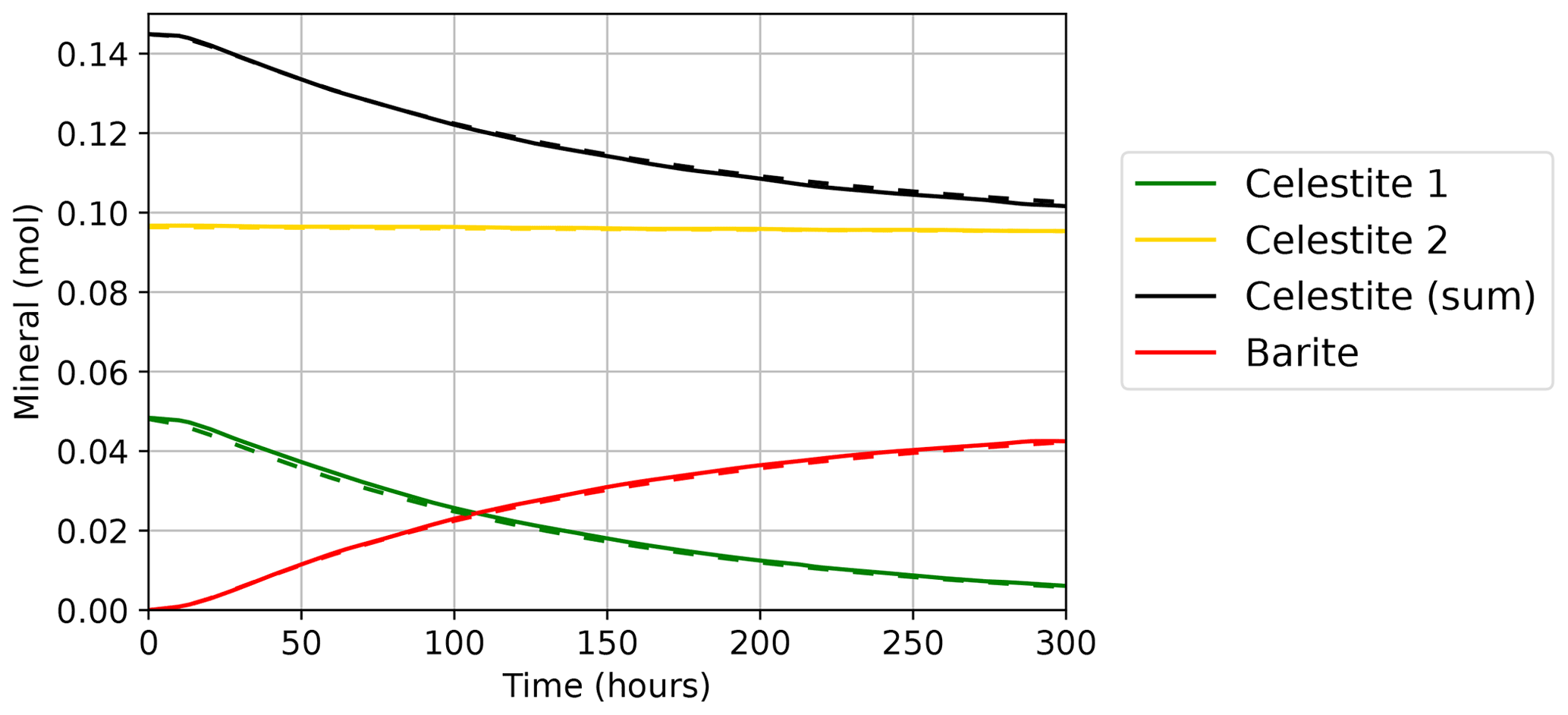
Figure 8 Temporal development of the mineral composition in the flow cell calculated by TRANSPORTSE-PHREEQC (dashed lines) in comparison against the results documented by Poonoosamy et al. (2021) (solid lines).

In view of Case 3b, Q2 is narrower with 0.005 m instead of 0.01 m ($\mathrm{0.045}\mathrm{m}\le x\le \mathrm{0.05}\mathrm{m}$), so that Q3 becomes accordingly wider. The initial porosity in Q2 is 10 % instead of 33 % and the initial permeability amounts to $\mathrm{5}\times {\mathrm{10}}^{-\mathrm{16}}$ m². Here, Q2 entirely consists of small celestite grains with a reactive surface area of 20 000 m² m⁻³, so that the lower porosity induces an overall higher surface area, and thus a faster dissolution and stronger decrease in porosity. The total simulation time amounts to 200 h.

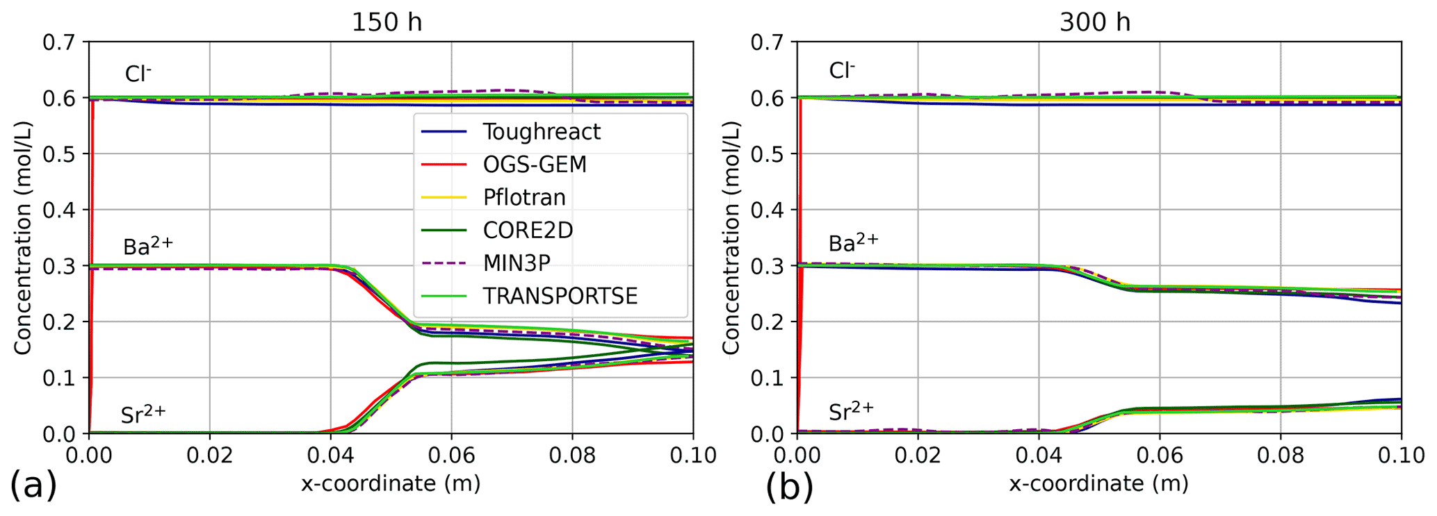
Figure 9 Ion concentrations along Line 1 at simulation times of (a) 150 h and (b) 300 h calculated by TRANSPORTSE-PHREEQC in comparison against the results documented by Poonoosamy et al. (2021).

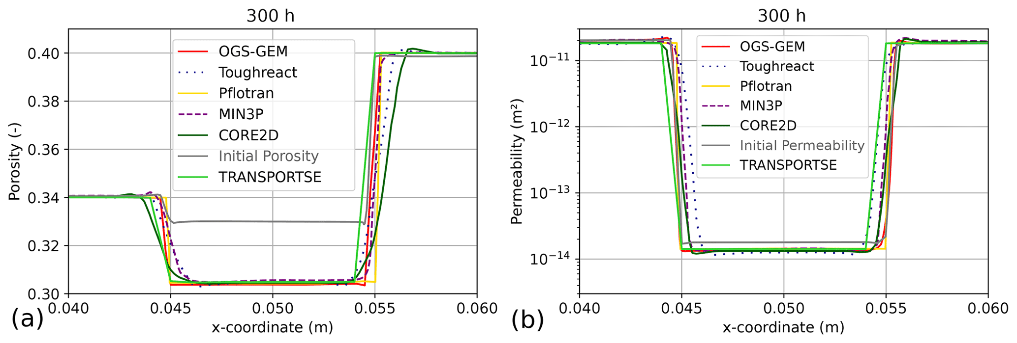
Figure 10 Calculated (a) porosity and (b) permeability changes along Line 1 at a simulation time of 300 h calculated by TRANSPORTSE-PHREEQC in comparison against the results documented by Poonoosamy et al. (2021).

3 Results and Discussions

Simulation results produced with TRANSPORTSE-PHREEQC for the two benchmarks are discussed in the following subsections by comparing these against the published reference data.

3.1 Engesgaard and Kipp (1992) Benchmark

As illustrated in Fig. 2, the profiles for concentrations, minerals and pH calculated with TRANSPORTSE-PHREEQC are in excellent agreement with the reference benchmark produced with a PHREEQC-based 1D advection and reactive transport model. The development of all curves is perfectly captured without any notable deviations. Consequently, it can be stated that the coupling between TRANSPORTSE and PHREEQC is verified for the advective transport benchmark, i.e. proofing that the internal calculation routines implemented in the chemical reaction function of the TRANSPORTSE configuration file correctly represent the chemical reactions and maintain the overall mass balances. This is a necessary condition for the further development of the coupling by increasing its overall complexity with the next benchmarks.

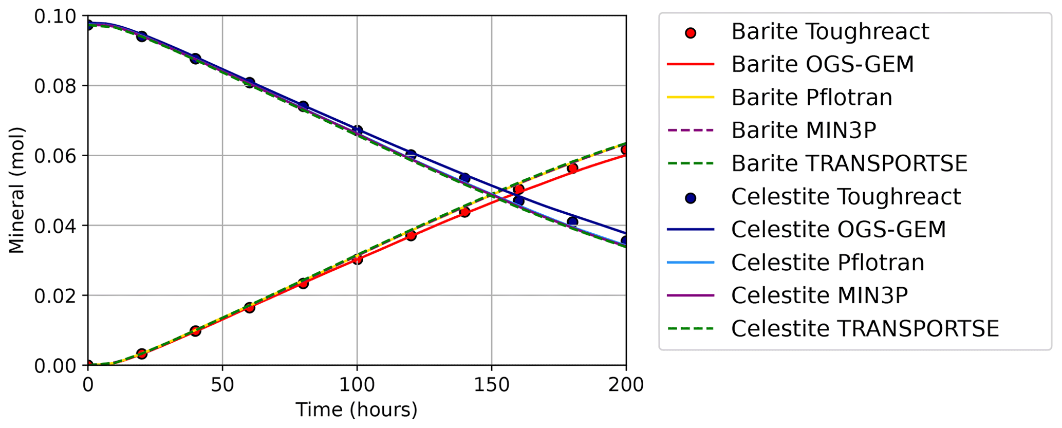
Figure 11 Temporal development of the mineral composition in the flow cell calculated by TRANSPORTSE-PHREEQC in comparison against the results documented by Poonoosamy et al. (2021).

3.2 Poonoosamy et al. (2021) Benchmarks

The Poonoosamy et al. (2021) benchmarks are discussed for the Cases 1, 2, 3a and 3b in the following, whereby model complexity is increasing with higher case numbers.

3.2.1 Case 1 – Conservative Mass Transport

Regarding Case 1, the flow field is very well reproduced, shown by a qualitative comparison of the reference  (Poonoosamy et al., 2021, Fig. 3) and TRANSPORTSE-PHREEQC (Fig. 3) simulation results.

Figure 4 shows that the time-dependent tracer amount in the model is also very well reproduced by TRANSPORTSE-PHREEQC, whereby the match against the MIN3P-THCm simulator is in a better agreement at the beginning than that against OpenGeoSys-GEM. The slightly higher initial tracer mass found in the TRANSPORTSE-PHREEQC results is due to the 3 g L⁻¹ concentration assigned to the three inlet elements, which were also considered in the overall mass balance calculation. Slight differences in the total tracer mass towards the end of the simulation time are likely related to numerical dispersion effects produced by the different discretisation methods (TRANSPORTSE – finite difference, MIN3P – finite volume and OGS – finite element) used by the three numerical codes as well as code-specific differences in the implementation of the outlet boundary conditions.

Figure 5 shows the temporal development of the tracer concentration in the flow cell at the observation points (c) and (d), respectively (see Fig. 1). The TRANSPORTSE-PHREEQC-based tracer concentration at point (c) starts increasing after about 10 h and is well in between those calculated by all other simulators (Fig. 5). This also holds true for the end of the simulation time at 24 h. At about 20 h, the TRANSPORTSE-PHREEQC results exhibit the lowest calculated concentration at its peak, however, it is still close to that calculated by MIN3P-THCm.

With regard to observation point (d), the tracer concentration calculated by TRANSPORTSE-PHREEQC is at the average of all other results in the beginning, and becomes the lowest one at a simulation time of 12–15 h, exhibiting a relatively good agreement with the PFLOTRAN simulation results. Towards the end of the simulation time at 15–19 h, the calculated concentration shows average values again, while it is above the other calculated ones at the end of the simulation.

In summary, a good agreement is achieved between the reference simulation and the results produced by TRANSPORTSE-PHREEQC. Consequently, this benchmark verifies that conservative mass transport is correctly implemented in the presented coupling in addition to the Engesgaard and Kipp (1992) benchmark. The new process considered here is hydrodynamic dispersion. Nevertheless, simulations without dispersion showed that its influence is relatively small, even though Poonoosamy et al. (2021) suggest that differences in the specific implementations may be the main reason for deviations in the simulation results between the different codes.

3.2.2 Case 2 – Density-driven Flow

Also for Case 2, the spatial distribution of the tracer concentration is very well reproduced (Fig. 6) in comparison to that presented by Poonoosamy et al. (2021, Fig. 8). The calculated fluid density at observation point (c) agrees very well with the Poonoosamy et al. (2021) data, especially for the MIN3P-Pitzer simulations (Fig. 7a).

Figure 7b shows that the fluid density calculated by TRANSPORTSE-PHREEQC at observation point (d) starts to increase later as for MIN3P-THCm and MIN3P-Pitzer. After 17–21 h, the calculated fluid density is lower than that derived from the other simulations and at the average at the end of the simulation time. The differences may result from the density calculation methods applied in the single codes, e.g., molar volumes may differ in the used databases, some codes use empirical relationships, and further there are also differences in the implementation of algorithms for diffusive-dispersive transport.

Consequently, also the coupling with respect to density-driven transport is verified. Our tests showed that the accuracy is sufficient even without the application of inner iterations. However, the chemical time step needs to be chosen carefully, as a decoupling is observed if flow and chemical time steps diverge.

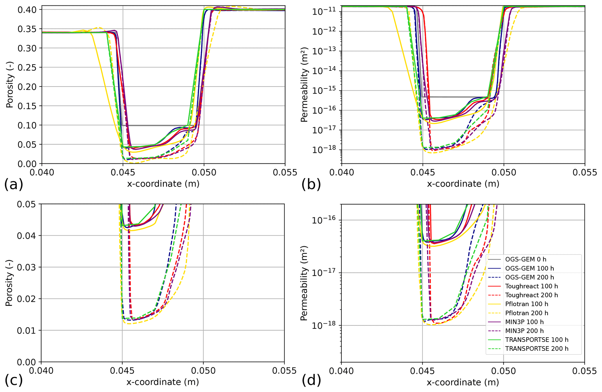
Figure 12 (a), (c) Porosity and (b), (d) permeability along the relevant Line 1 section in the flow cell at simulation times of 100 and 200 h calculated by TRANSPORTSE-PHREEQC in comparison against the results documented by Poonoosamy et al. (2021).

3.2.3 Case 3a – Reactive Transport with low Porosity Changes

Figure 8 shows that the calculated mineral amounts in the flow cell agree well with the reference data. The initial amount of celestite calculated by TRANSPORTSE-PHREEQC is slightly lower, which may result from different input data related to densities and/or molar volumes. In the long-term, the amount of celestite is slightly higher, while the barite amount is accordingly lower. This is assumed to result from a lower celestite conversion due to minor differences related to dispersive transport. Nevertheless, the deviations are negligible in the authors' view.

The concentrations after 150 h simulated with TRANSPORTSE-PHREEQC (Fig. 9a) agree very well with the results documented by Poonoosamy et al. (2021). Those for Cl and Ba are comparably high, while the Sr concentration is found in between the other curves. This behaviour has been also observed for Case 1, where concentrations become average in comparison to the other simulation results.

Figure 9b shows the concentrations calculated for a simulation time of 300 h. Here, the Cl concentration is rather at the upper limit compared to the reference data, while all other species are at average values.

The temporal porosity evolution is presented in Fig. 10a and shows a good agreement with the other simulation results. Differences at the interfaces between regions Q1–Q2 and Q2–Q3 are probably resulting from the curve fitting functions applied by Poonoosamy et al. (2021), which obviously produce overshooting in the reference data.

Figure 10b shows the permeability along Line 1, which is in good agreement with the reference simulation results. Again, differences in some of the simulation results presented by Poonoosamy et al. (2021) result from a poor choice of the applied curve fitting functions.

In summary for Case 3a, the TRANSPORTSE-PHREEQC coupling is also verified with respect to porosity and permeability changes due to mineral precipitation and dissolution.

3.2.4 Case 3b – Reactive Transport with high Porosity Changes

Preliminary simulations of Case 3b showed that the solution volume needs to be adapted to changes in pore volume. Otherwise, the dissolution of celestite occurs too fast due to the smaller increase in saturation, and thus higher dissolution rate. If the water volume in the pores is accordingly adapted, the mineral amounts presented in Fig. 11 agree very well, especially in view of the results produced by MIN3P-THCm and PFLOTRAN.

Figure 12 shows the porosity and permeability along Line 1 at 100 and 200 h, respectively. A good agreement is achieved for both simulation times, whereby the TRANSPORTSE-PHREEQC results generally range in between the curves produced by the other numerical codes.

In view of the very good agreement with the reference data, it can be concluded that the TRANSPORTSE-PHREEQC coupling is also verified in terms of the reactive transport benchmark involving high porosity changes.

4 Conclusions

The present study demonstrates the successful verification of the TRANSPORTSE-PHREEQC coupling implementation. For that purpose, two computationally challenging benchmarks have been employed to assess the coupling between purely advective transport and chemical reactions as well as a step-wise increase in model complexity. Thereby, effects of density-driven flow as well as porosity and permeability changes were introduced with increasing computational demand. The overall results show a very good agreement with the reference data with negligible deviations which may be explained by the different code implementations (e.g., for hydrodynamic dispersion) used by the different code authors. Further challenges in reactive transport modelling remain, including the maintenance of fluid volume balances with changes in porosity resulting from mineral dissolution and precipitation. These may be addressed by the implementation of specific source and sink terms for the respective model elements in upcoming studies.

In summary, the present contribution introduces an extension of the Open Source and Open Access TRANSPORT Simulation Environment (Kempka, 2020) which is now capable to solve reactive transport problems, allowing users with limited software development skills to flexibly adapt fluid and rock equations of state, chemical reaction modules used for reactive transport, dynamic boundary conditions and mass balance calculations to their specific requirements. Further, it was demonstrated that the computationally demanding benchmarks introduced by Poonoosamy et al. (2021) can be also successfully reproduced with the PHREEQC code, coupled to a suitable fluid flow and chemical species transport simulator.

Future work will focus on application of the verified TRANSPORTSE-PHREEQC implementation to different scientific questions which require the flexible implementation of arbitrary thermo-hydro-geochemical systems, such as groundwater resource management, permafrost degradation, geological energy storage, nuclear waste storage, etc.