TransPyREnd: a code for modelling the transport of radionuclides on geological timescales

The German site selection procedure for a high-level nuclear waste repository is entering a stage in which preliminary safety assessments have to be conducted and the release of radionuclides has to be estimated for a large number of potential sites.

Here, we present TransPyREnd, a 1D finite-differences code for modeling the transport of radionuclides in the subsurface at geological timescales. The code simulates the processes advection, diffusion, equilibrium sorption, decay of radionuclides, and the build-up of daughter nuclides. We summarize the modeled physical processes, their mathematical description and our numerical approach to solve the governing equations. Finally, two simple tests are shown, one considering diffusion, sorption, and radioactive decay, the other involving diffusion and a radioactive decay chain. In both tests, the code shows good agreement with the reference solutions. Caveats of the model and future additions are discussed.

1 Introduction

In the German site selection procedure for a high-level nuclear waste repository preliminary safety assessments have to be evaluated in three consecutive phases. In the first phase (starting 2020) representative preliminary safety assessments have to be carried out for a large number of potential sites (Hoyer et al., 2021; StandAG, 2017), with three different types of host rock considered (clay rock, rock salt, crystalline rock). The legal requirements include strict criteria on both the maximum mass and the maximum amount of radionuclides that are allowed to be released from the repository or its surroundings over one million years (10⁻⁴ of the total mass and amount initially disposed), and a maximum rate of release (10⁻⁹ yr⁻¹ of the total mass and amount initially disposed). These criteria need to be evaluated individually for each potential site. The detailed legal requirements can be found in EndlSiAnfV (2020) (Disposal Safety Requirements Ordinance) and StandAG (2017) (Repository Site Selection Act).

In general, the large number of radionuclides to consider (several hundreds up to a thousand) make such evaluations difficult. Apart from the complexity of considering three different types of host rock, the particular challenge in the German site selection procedure is two-fold: First, the number (and area) of potential sites is large, with 54 % of the area of Germany being a potential site after the initial stage of the site selection procedure (BGE, 2020). Secondly, data for parametrizing transport/reaction models is both heterogeneous and scarce. Some geological information and basic parameters such as porosity may be available site-specific from different sources. However, other parameters governing the details of the transport process are widely unavailable from local measurements and need to be estimated in a systematic way, as on-site exploration/measurements will only begin in subsequent stages of the site selection procedure. Given the sparse data, it is beneficial to employ a computationally efficient 1D code that can be used to run large sets of models in order to capture the uncertainties in the governing parameters.

At present, a workflow for estimating the transport parameters is set up, which is inspired by the one developed by Nagra for the Swiss site selection procedure (Van Loon, 2014, note that these authors focus on clay formations only). Details can be found in BGE (2022a).

In the literature, several models and codes for assessing the migration of radionuclides out of a deposit exist, e.g. Norman and Kjellbert (1990), Reiche (2016), Nagra (2013), Garibay-Rodriguez et al. (2022), Trinchero et al. (2020). For the safety assessments in the German site selection procedure, one constraint was the desire to be able to publish the code as open-source. Additional requirements for the code include simplicity, ease of use, and performance. The code should be light-weight and should not rely on large third-party tools to reduce the complexity. In the version presented here, the code focuses on porous media and does not include a treatment of fractured media, which could be important for transport in crystalline rocks.

Our transport model for the representative preliminary safety assessments and its implementation is named TransPyREnd (“Transportmodell in Python für Radionuklide aus einem Endlager”, English translation “Transport model in Python for radionuclides in a nuclear waste repository”). It will be released as an open-source project in early 2023, and will provide a unique opportunity for the community and public to assess the model, test and/or modify it. This will both help in assuring quality of the tools used in the site selection procedure, and aid in trust-building for the general public.

Model approach

A number of choices have to be made to develop a model for the transport of radionuclides. Here only one spatial dimension (1D) is considered, that is, we model transport along a line, e.g. in the vertical, horizontal, or any other meaningful direction. Given the limited available data and the large number of potential sites, this is a justified approximation also applied in other safety assessments, e.g. Nagra (2002). A 1D model also has advantages in terms of the low computational effort needed. Hence, uncertainties can easily be incorporated in the parametrization by evaluating ensembles of model runs, i.e. sets of models in which uncertainties are accounted for by varying the parameters within a distinct range. The general concept of dealing with uncertainties in the preliminary safety assessments can be found in BGE (2022b). In short, the workflows used for generating the model parameters are also used to estimate the uncertainties in these parameters. Sensitivity analyses are used to assess which parameters are important: the combined uncertainties in sensitive parameters are then evaluated using Monte-Carlo simulations.

Furthermore, the scope of the model is limited to the transport through the geological barriers far from the emplacement area (also termed as the “far-field” in contrast to the “near-field” that would include the technical barriers near the emplacement area). The transport along e.g. mining shafts or other technical elements is currently not included in the model.

Transport is included in the host rock layer and in geological layers above and below (if transport is vertical) or next (in case of horizontal transport) to the host rock layer. A sketch of an example model domain for vertical transport is shown in Fig. 1. As the current application is limited to the question of how much of the disposed radionuclides escape from the host rock, following the legal and regulatory demands (EndlSiUntV, 2020), what we extract from the completed model is the amount and mass of radionuclides released from the host rock layer. Nevertheless, the model contains all relevant geological layers, as these have an effect on the release from the host rock.

Regarding the modeled processes, diffusion, advection, mechanical dispersion, and sorption are considered. Diffusion is assumed to be Fick'ian (Tartakovsky and Dentz, 2019), and differing accessible porosities (Van Loon, 2014) for individual nuclides (depending on whether they are present as anions or cations) are taken into account, assuming a fixed speciation. We assume Darcy's law holds for advection, as flow velocities in the host rock are expected to be very small due to the low hydraulic permeability expected in the host rocks (in particular in rock salt and clay). Consequently, the model is not applicable where turbulent flows are expected. All pore space is assumed to be saturated, following e.g. Nagra (2014). Ignoring the unsaturated zone introduces only a small error in most cases. In arid environments, the unsaturated zone might be very large, but even in this case, the assumption will still be conservative: It will lead to an overestimation of the radionuclide release, not to an underestimation. Dispersion can be included as an effectively increased diffusion. Sorption is modeled as linear equilibrium sorption (Freundlich, 1907), i.e. we do not consider competition for sorption sites.

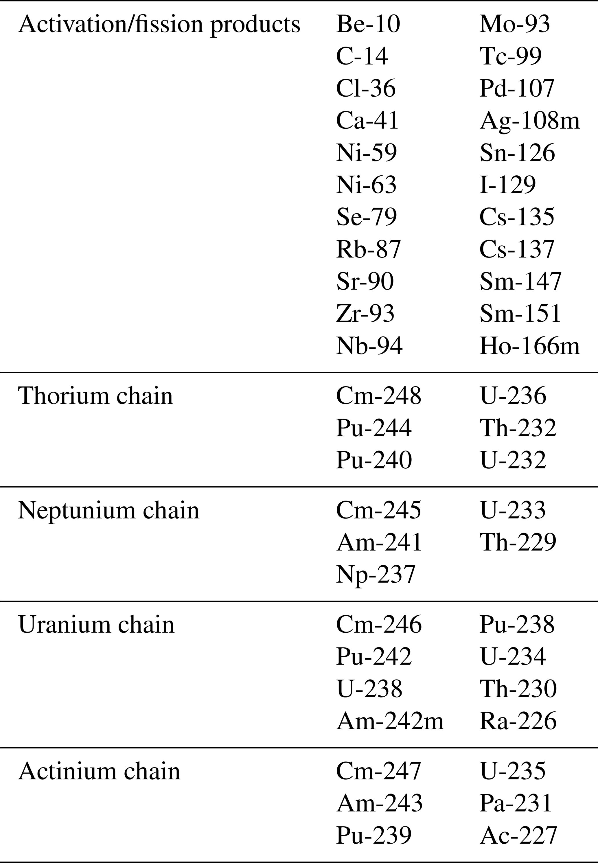
Additionally, we include radioactive decay and the formation of daughter nuclides, as required by the regulatory stipulations. The inventory of nuclear waste that has to be stored contains hundreds of different radionuclides: however, many of them can be shown to be not relevant for the effective release of radionclides. For example, a radionuclide with a half-life of hours will not be transported significantly in the designated host rock before it decays, even in a pessimistic scenario. However, its daughter nuclide might be relevant, if it has a long half-life. At present, a simplified nuclide scheme following this line of argument is employed, taking into account 47 radionuclides (Larue et al., 2013; Fischer-Appelt et al., 2013). It neglects nuclides with small half-lifes, but includes long-lived daughters of short-lived radionuclides. The 47 nuclides in the scheme are shown in Table 1.

Table 1 The nuclides included in the simplified nuclide scheme of Larue et al. (2013), Fischer-Appelt et al. (2013).

Several additional physical processes and their coupling are not taken into account which is discussed together with other simplifications at the end of Sect. 4.

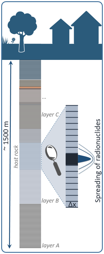
Figure 1 Schematic depiction of the model domain. Note that the direction of transport is not necessarily vertical as shown here. Note that while the zoom-in only shows the host rock, all geological layer are discretized.

2 Mathematical approach

2.1 Governing equations

The model computes the evolution of concentration c_i for each nuclide i over time.

The aforementioned processes can be included into a set of coupled differential equations, namely one equation for each of the n_s radionuclides considered. The 1D transport equation for the nuclide with the index i reads (compare i.e. Bear, 1972; de Marsily, 1986; Kinzelbach, 1992; Clauser, 2003):

$$\begin{array}{}\text{(1)}& \begin{array}{rl}\underset{\begin{array}{c}\text{Concentration}\\ \text{change}\end{array}}{\underbrace{\phantom{\sum _j}{\mathit{\varphi }}_i{R}_i{\displaystyle \frac{\partial c_i}{\partial t}}}}& ={\displaystyle \frac{\partial }{\partial x}}(\underset{\text{Diffusion}}{\underbrace{\phantom{\sum _j}{D}_{\mathrm{e},i}{\displaystyle \frac{\partial c_i}{\partial x}}}}-\underset{\text{Advection}}{\underbrace{\phantom{\sum _j}q{c}_i}})\\ & +\underset{\text{Decay}}{\underbrace{\phantom{\sum _j}\sum _j\left(R_j{\mathit{\varphi }}_i{c}_j{\mathit{\lambda }}_{i,j}\right)-R_i{\mathit{\varphi }}_i{c}_i{\mathrm{\Lambda }}_i}}+\underset{\text{Source term}}{\underbrace{\phantom{\sum _j}{W}_i}}\end{array}\end{array}$$

Here, c_i is the amount of nuclide i per fluid volume, measured in mol m⁻³. R_i is the retardation factor, defined as

$$\begin{array}{}\text{(2)}& R_i=\mathrm{1}+{\displaystyle \frac{K_{\mathrm{d},i}{\mathit{\rho }}_{\mathrm{b}}}{{\mathit{\varphi }}_i}},\end{array}$$

and is the factor by which sorption slows down transport due to advection and diffusion.

K_d,i is the linear equilibrium sorption coefficient, ρ_b is the bulk density of the rock, and ϕ_i is the accessible porosity. D_e,i is the effective diffusion coefficient,

$$\begin{array}{}\text{(3)}& D_{\mathrm{e},i}=D_i{\mathit{\varphi }}_i,\end{array}$$

with D_i being the diffusion coefficient for nuclide i. If an additional dispersion term is to be considered, D_e,i should be replaced by

$$\begin{array}{}\text{(4)}& D_{\mathrm{e},i}^{\star }=D_{\mathrm{e},i}+D_{\mathrm{disp}}\end{array}$$

with D_disp being the dispersion. λ_i,j is the reaction rate for the decay of nuclide j to nuclide i, and Λ_i is the total decay rate of nuclide i. The total decay rate Λ_i is related to the nuclide's half-life $t_{\mathrm{1}/\mathrm{2}}$ by ${\mathrm{\Lambda }}_i=\log \mathrm{2}{t}_{\mathrm{1}/\mathrm{2}}^{-\mathrm{1}}$. The individual rates λ_i,j are connected to this total decay rate by the branching fraction of the relevant decay channel. Finally, W_i is a generic source term for radionuclides, that is, it has units of amount of substance per volume and time and measures the inflow of radionuclides from an external source. This can be used, for example, to connect the model to a dedicated near field or canister release model. R_i appears on both sides of the equation, but not in front of the advective and diffusive terms, reflecting that it expresses the factor by which both advection and diffusion are reduced due to sorption. The decay term consists of a term with a positive sign, which measures the rate at which other nuclides decay into nuclide i, and a term with negative sign, measuring the rate at which nuclide i itself decays into other nuclides, including those that are not explicitly tracked in the model (e.g. individual stable nuclides).

Note that we consider transport in various geological layers, so the retardation factor R_i, effective diffusion coefficient K_d,i, and porosity ϕ_i are in general functions of location x. q is the Darcy velocity.

In the following, we do not consider steady state solutions to the system in Eq. (1). The physical problem we want to solve involves a finite total amout of radioactive waste, meaning that the steady-state solution is the trivial one in which all radionuclides have decayed to stable nuclides. Thus, we focus on the transient solution of the system of equations.

2.2 Numerical methods

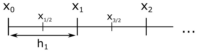
In order to solve Eq. (1), we resort to a numerical treatment via a finite difference scheme. The finite difference method is a well established method for solving ordinary and partial differential equations (i.e. Shamir and Harleman, 1967; Marsal, 1989; Clauser, 2003; Rühaak et al., 2008; Luijendijk, 2012). We divide our domain into n nodes at location x_k. The distance between grid points, $h_k=x_k-x_{k-\mathrm{1}}$ is allowed to vary in space. An illustration of the grid structure is shown in Fig. 2.

Figure 2 Illustration of the grid structure.

Accordingly, the transient problem in the time domain is split into specific time-steps.

The solution of transient partial differential equations requires initial and boundary conditions.

2.2.1 Discretization of derivatives

We begin by writing down discretized approximations of the right hand side of Eq. (1). As mentioned before we assume D_e to vary with location, whereas q is assumed to be constant. In the following, we use the index k to denote the node at which we evaluate a quantity. As expected, special treatment of the boundary nodes (k=0, $k=n-\mathrm{1}$) is necessary.

For the diffusive term, we use the following central difference scheme (e.g. LeVeque, 2007):

$$\begin{array}{}\text{(5)}& \begin{array}{rl}{\displaystyle \frac{\partial }{\partial x}}{D}_{\mathrm{e},i}{\displaystyle \frac{\partial c}{\partial x}}& \approx {\displaystyle \frac{\mathrm{2}}{h_{k+\mathrm{1}}+h_k}}\left({\displaystyle \frac{\mathrm{1}}{h_k}}{D}_{\mathrm{e},i,k-\frac{\mathrm{1}}{\mathrm{2}}}{c}_{i,k-\mathrm{1}}\right.\\ & -{\displaystyle \frac{h_{k+\mathrm{1}}+h_k}{h_k{h}_{k+\mathrm{1}}}}\left(D_{\mathrm{e},i,k-\frac{\mathrm{1}}{\mathrm{2}}}+D_{\mathrm{e},i,k+\frac{\mathrm{1}}{\mathrm{2}}}\right)c_{i,k}\\ & \left.+{\displaystyle \frac{\mathrm{1}}{h_{k+\mathrm{1}}}}{D}_{\mathrm{e},i,k+\frac{\mathrm{1}}{\mathrm{2}}}{c}_{i,k+\mathrm{1}}\right)\end{array}\end{array}$$

Here, the index $k\pm \frac{\mathrm{1}}{\mathrm{2}}$ denotes the location half-way between node k and node k±1, $x_{k\pm \mathrm{1}/\mathrm{2}}$. The diffusion coefficient at these interfaces is evaluated using a harmonic mean (Huysmans and Dassargues, 2007). Clearly, in the case of a homogeneous diffusion coefficient and a constant grid spacing h_k=h, Eq. (5) reduces to the familiar second order central difference.

The advection term is also approximated using central differences:

$$\begin{array}{}\text{(6)}& q{\displaystyle \frac{\partial c}{\partial x}}\approx q{\displaystyle \frac{c_{i,k+\mathrm{1}}-c_{i,k-\mathrm{1}}}{x_{k+\mathrm{1}}-x_{k-\mathrm{1}}}}\end{array}$$

Evaluation of the decay and source term in Eq. (1) is straight-forward, as they do not include derivatives.

2.2.2 Time-evolution scheme

To solve the equation, we need to choose a time-evolution scheme. We use a semi-implicit scheme governed by a meta parameter $\mathrm{0}\le \mathit{\theta }\le \mathrm{1}$ sometimes called the θ-method as it is robust and relatively fast.

The θ-method is a one-step scheme and a combination of the Euler forwards and backwards schemes. For θ=0.5 it becomes the second-order accurate Crank-Nicolson scheme (Crank and Nicolson, 1947). Schematically, for a given differential equation of the form

$$\begin{array}{}\text{(7)}& {\displaystyle \frac{\partial y}{\partial t}}=f(x,y,t)\end{array}$$

the θ-scheme yields

$$\begin{array}{}\text{(8)}& {\displaystyle \frac{y^{m+\mathrm{1}}-y^m}{\mathrm{\Delta }t}}=\mathit{\theta }{F}^{m+\mathrm{1}}+(\mathrm{1}-\mathit{\theta })F^m\end{array}$$

where F is an appropriate discretization of f, and where we use the index m to denote the discrete time step m at which a quantity is evaluated. For θ=0, this becomes the Euler-forwards scheme which is prone to numerical instability. For θ=1, it becomes the Euler-backwards scheme which is unconditionally stable, and for θ=0.5 we recover the Crank-Nicolson scheme which is second order accurate and unconditionally stable as well.

Inserting our discretizations from Eqs. (5) and (6), as well as the decay and source term into Eq. (8), we obtain:

$$\begin{array}{ll}{\displaystyle }{R}_{i,k}{\mathit{\varphi }}_{i,k}{\displaystyle \frac{c_{i,k}^{m+\mathrm{1}}-c_{i,k}^m}{\mathrm{\Delta }t}}& {\displaystyle }=\mathit{\theta }{H}_k\left(H_k^{-}{D}_{\mathrm{e},i,k-\frac{\mathrm{1}}{\mathrm{2}}}{c}_{i,k-\mathrm{1}}^{m+\mathrm{1}}\right.\\ {\displaystyle }& {\displaystyle }-G_k\left(D_{\mathrm{e},i,k-\frac{\mathrm{1}}{\mathrm{2}}}+D_{\mathrm{e},i,k+\frac{\mathrm{1}}{\mathrm{2}}}\right)c_{i,k}^{m+\mathrm{1}}\\ {\displaystyle }& {\displaystyle }\left.+H_k^{+}{D}_{\mathrm{e},i,k+\frac{\mathrm{1}}{\mathrm{2}}}{c}_{i,k+\mathrm{1}}^{m+\mathrm{1}}\right)\\ {\displaystyle }& {\displaystyle }-\mathit{\theta }q{\displaystyle \frac{c_{i,k+\mathrm{1}}^{m+\mathrm{1}}-c_{i,k-\mathrm{1}}^{m+\mathrm{1}}}{x_{k+\mathrm{1}}-x_{k-\mathrm{1}}}}\\ {\displaystyle }& {\displaystyle }+(\mathrm{1}-\mathit{\theta })H_k\left(H_k^{-}{D}_{\mathrm{e},i,k-\frac{\mathrm{1}}{\mathrm{2}}}{c}_{i,k-\mathrm{1}}^m\right.\\ {\displaystyle }& {\displaystyle }-G_k\left(D_{\mathrm{e},i,k-\frac{\mathrm{1}}{\mathrm{2}}}+D_{\mathrm{e},i,k+\frac{\mathrm{1}}{\mathrm{2}}}\right)c_{i,k}^m\\ {\displaystyle }& {\displaystyle }\left.+H_k^{+}{D}_{\mathrm{e},i,k+\frac{\mathrm{1}}{\mathrm{2}}}{c}_{i,k+\mathrm{1}}^m\right)\\ {\displaystyle }& {\displaystyle }-(\mathrm{1}-\mathit{\theta })q{\displaystyle \frac{c_{i,k+\mathrm{1}}^m-c_{i,k-\mathrm{1}}^m}{x_{k+\mathrm{1}}-x_{k-\mathrm{1}}}}\\ {\displaystyle }& {\displaystyle }+\sum _j\left(R_{j,k}{\mathit{\varphi }}_{j,k}{c}_{j,k}^m{\mathit{\lambda }}_{i,j}\right)\\ \text{(9)}& {\displaystyle }& {\displaystyle }-R_{i,k}{\mathit{\varphi }}_{i,k}{c}_{i,k}^m{\mathrm{\Lambda }}_i+W_{i,k}^m\end{array}$$

Where we have defined

$$\begin{array}{}\text{(10)}& {\displaystyle }{H}_k& {\displaystyle }={\displaystyle \frac{\mathrm{2}}{h_{k+\mathrm{1}}+h_k}}\text{(11)}& {\displaystyle }{H}_k^{-}& {\displaystyle }={\displaystyle \frac{\mathrm{1}}{h_k}}\text{(12)}& {\displaystyle }{H}_k^{+}& {\displaystyle }={\displaystyle \frac{\mathrm{1}}{h_{k+\mathrm{1}}}}\text{(13)}& {\displaystyle }{G}_k& {\displaystyle }={\displaystyle \frac{h_{k+\mathrm{1}}+h_k}{h_k{h}_{k+\mathrm{1}}}}\end{array}$$

As can be seen from Eq. (9), the decay terms are evaluated at time step m and not m+1, like the additional external source term. This is necessary to deal with the dependency of c_i on potentially all other c_j with j≠i that could decay into c_i. As the currently used nuclide chains are relatively simple, it would be possible to sort the equations in a way that allows including the decay term in an implicit fashion. We leave this to future work. By defining

$$\begin{array}{}\text{(14)}& {\displaystyle }s& {\displaystyle }={\displaystyle \frac{\mathrm{\Delta }t}{{\mathit{\varphi }}_{i,k}{R}_{i,k}}}\text{(15)}& {\displaystyle }{u}_k& {\displaystyle }={\displaystyle \frac{qs}{x_{k+\mathrm{1}}-x_{k-\mathrm{1}}}}\text{(16)}& {\displaystyle }{v}_k^{-}& {\displaystyle }=H_k{H}_k^{-}{D}_{\mathrm{e},i,k-\mathrm{1}/\mathrm{2}}s\text{(17)}& {\displaystyle }{v}_k& {\displaystyle }=H_k{G}_k(D_{\mathrm{e},i,k-\mathrm{1}/\mathrm{2}}+D_{\mathrm{e},i,k+\mathrm{1}/\mathrm{2}})s\text{(18)}& {\displaystyle }{v}_k^{+}& {\displaystyle }=H_k{H}_k^{+}{D}_{\mathrm{e},i,k+\mathrm{1}/\mathrm{2}}s\text{(19)}& {\displaystyle }{\mathit{\theta }}^{\prime }& {\displaystyle }=\mathrm{1}-\mathit{\theta }\end{array}$$

and rearranging the terms in Eq. (9) such that unknown terms are on the left, we find

$$\begin{array}{ll}{\displaystyle }& {\displaystyle }\mathit{\theta }\left(-u_k-v_k^{-}\right)c_{i,k-\mathrm{1}}^{m+\mathrm{1}}+\left(\mathrm{1}+\mathit{\theta }{v}_k\right)c_{i,k}^{m+\mathrm{1}}\\ {\displaystyle }& {\displaystyle }+\mathit{\theta }\left(u_k-v_k^{+}\right)c_{i,k+\mathrm{1}}^{m+\mathrm{1}}=\\ {\displaystyle }& {\displaystyle }{\mathit{\theta }}^{\prime }\left(u_k+v_k^{-}\right)c_{i,k-\mathrm{1}}^m+\left(\mathrm{1}-{\mathit{\theta }}^{\prime }{v}_k\right)c_{i,k}^m\\ {\displaystyle }& {\displaystyle }+{\mathit{\theta }}^{\prime }\left(-u_k+v_k^{+}\right)c_{i,k+\mathrm{1}}^m\\ \text{(20)}& {\displaystyle }& {\displaystyle }+s\left(\sum _j\left(R_j{\mathit{\varphi }}_i{c}_{j,k}^m{\mathit{\lambda }}_{i,j}\right)-R_i{\mathit{\varphi }}_i{c}_{i,k}^m{\mathrm{\Lambda }}_i+W_{i,k}^m\right)\end{array}$$

2.2.3 Matrix equation

Identifying the right hand side with a vector b, this can be represented as a matrix equation, ${\mathbf{M}}_i{\mathit{c}}_i^{m+\mathrm{1}}={\mathit{b}}_i$, for each nuclide i. M_i is a tridiagonal matrix with the structure:

$$\begin{array}{}\text{(21)}& \begin{array}{rl}& {\mathbf{M}}_i=\\ & \left[\begin{array}{ccccccc}{B}_{\mathrm{l},\mathrm{0}}& B_{\mathrm{l},\mathrm{1}}& \mathrm{0}& \mathrm{\dots }& \mathrm{\dots }& \mathrm{\dots }& \mathrm{\dots }\\ \mathit{\theta }(-u_{\mathrm{1}}-v_{\mathrm{1}}^{-})& \mathrm{1}+\mathit{\theta }{v}_{\mathrm{1}}& \mathit{\theta }(u_{\mathrm{1}}-v_{\mathrm{1}}^{+})& \mathrm{0}& \mathrm{\dots }& \mathrm{\dots }& \mathrm{\dots }\\ \mathrm{0}& \mathit{\theta }(-u_{\mathrm{2}}-v_{\mathrm{2}}^{-})& \mathrm{1}+\mathit{\theta }{v}_{\mathrm{2}}& \mathit{\theta }(u_{\mathrm{2}}-v_{\mathrm{2}}^{+})& \mathrm{0}& \mathrm{\dots }& \mathrm{\dots }\\ \mathrm{\dots }& \mathrm{\dots }& \mathrm{\dots }& \mathrm{\dots }.& \mathrm{\dots }& \mathrm{\dots }& \mathrm{\dots }\\ \mathrm{\dots }& \mathrm{\dots }& \mathrm{\dots }& \mathrm{0}& \mathit{\theta }(-u_{\mathrm{n}-\mathrm{2}}-v_{\mathrm{n}-\mathrm{2}}^{-})& \mathrm{1}+\mathit{\theta }{v}_{\mathrm{n}-\mathrm{2}}& \mathit{\theta }(u_{\mathrm{n}-\mathrm{2}}-v_{\mathrm{n}-\mathrm{2}}^{+})\\ \mathrm{\dots }& \mathrm{\dots }& \mathrm{\dots }& \mathrm{\dots }& \mathrm{0}& B_{\mathrm{r},\mathrm{n}-\mathrm{2}}& B_{\mathrm{r},\mathrm{n}-\mathrm{1}}\end{array}\right]\end{array}\end{array}$$

The terms B_l,0, B_l,1, $B_{\mathrm{r},\mathrm{n}-\mathrm{2}}$, $B_{\mathrm{r},\mathrm{n}-\mathrm{1}}$ control how the boundary nodes – the nodes on the left and right edge of the model domain – evolve and are set by the boundary conditions.

Again, it becomes evident here why we treat the decay terms as an external source term evaluated at time step m: otherwise, we could not write the equation as system of linear equations, because the decay term couples the concentration of different species with each other.

2.2.4 Boundary conditions

Dirichlet boundary conditions are used to fix the concentration at the outer edges of the domain (here termed left and right) to a constant value, i.e. $c_{i,\mathrm{0}}^m=c_{i,\mathrm{0}}^{m+\mathrm{1}}=C_{i,\mathrm{left}},c_{i,\mathrm{n}-\mathrm{1}}^m=c_{i,\mathrm{n}-\mathrm{1}}^{m+\mathrm{1}}=C_{i,\mathrm{right}}$ yielding:

$$\begin{array}{}\text{(22)}& {\displaystyle }{B}_{\mathrm{l},\mathrm{0}}=\mathrm{1},B_{\mathrm{l},\mathrm{1}}=\mathrm{0},B_{\mathrm{r},\mathrm{n}-\mathrm{2}}=\mathrm{0},B_{\mathrm{r},\mathrm{n}-\mathrm{1}}=\mathrm{1}\end{array}$$

and the vector entries are set to the specified concentrations, $b_{\mathrm{0}}=C_{i,\mathrm{left}}$ or $b_{\mathrm{n}-\mathrm{1}}=C_{i,\mathrm{right}}$.

Neumann boundary conditions can be considered as well. For the left boundary at k=0, they are defined by

$$\begin{array}{}\text{(23)}& {\displaystyle \frac{\partial c_i}{\partial x}}{|}_{x=\mathrm{0}}=j_{\mathrm{l}}\approx {\displaystyle \frac{c_{i,\mathrm{1}}^m-c_{i,-\mathrm{1}}^m}{\mathrm{2}{h}_{\mathrm{0}}}},\end{array}$$

where we have applied a central differencing scheme on the right hand side. The node at $k=-\mathrm{1}$ is a fictitious grid point outside of the domain, and we set h₀=h₁. Furthermore, we assume $D_{k_{-}\frac{\mathrm{1}}{\mathrm{2}}}=D_{k_{+}\frac{\mathrm{1}}{\mathrm{2}}}$.

We can use Eq. (23) to eliminate the fictitious grid point from the transport equation for the boundary, which results in

$$\begin{array}{ll}{\displaystyle }& {\displaystyle }\left(\mathrm{1}+\mathrm{2}\mathit{\theta }{v}_{\mathrm{0}}^{+}\right)c_{i,\mathrm{0}}^{m+\mathrm{1}}+\left(-\mathrm{2}\mathit{\theta }{v}_{\mathrm{0}}^{+}\right)c_{i,\mathrm{1}}^{m+\mathrm{1}}=\\ \text{(24)}& {\displaystyle }& {\displaystyle }\left(\mathrm{1}-\mathrm{2}{\mathit{\theta }}^{\prime }{v}_{\mathrm{0}}^{+}\right)c_{i,\mathrm{0}}^m+\left(\mathrm{2}{\mathit{\theta }}^{\prime }{v}_{\mathrm{0}}^{+}\right)c_{i,\mathrm{1}}^m-\mathrm{2}{h}_{\mathrm{0}}{j}_{\mathrm{l}}\left(u_{\mathrm{0}}+v_{\mathrm{0}}^{+}\right)+\mathrm{\dots }\end{array}$$

where we have omitted the decay and source terms for brevity. Consequently, the boundary terms for Neumann boundary conditions on the left boundary read:

$$\begin{array}{}\text{(25)}& \begin{array}{rl}{B}_{\mathrm{l},\mathrm{0}}& =\mathrm{1}+\mathrm{2}\mathit{\theta }{v}_{\mathrm{0}}^{+},B_{\mathrm{l},\mathrm{1}}=-\mathrm{2}\mathit{\theta }{v}_{\mathrm{0}}^{+}\\ b_{\mathrm{0}}& =\left(\mathrm{1}-\mathrm{2}{\mathit{\theta }}^{\prime }{v}_{\mathrm{0}}^{+}\right)c_{i,\mathrm{0}}^m+\left(\mathrm{2}{\mathit{\theta }}^{\prime }{v}_{\mathrm{0}}^{+}\right)c_{i,\mathrm{1}}^m\\ & -\mathrm{2}{h}_{\mathrm{0}}{j}_{\mathrm{l}}\left(u_{\mathrm{0}}+v_{\mathrm{0}}^{+}\right)+\mathrm{\dots }\end{array}\end{array}$$

A similar derivation can be made for Neumann boundaries on the right boundary of the model.

2.2.5 Initial conditions

We assume instantaneous release of the radionuclides from canisters and the emplacement area and neglect solubility limits. Thus, the initial conditions are simply given by the total amount of each radionuclide in the repository and the volume of the repository. Future development will be focused on overcoming this simplification, see Sect. 4.

2.2.6 Implementation

The matrix Eq. (21) can be solved using standard methods. Our implementation is based on the PyBasin model (Luijendijk, 2020).

Given the sparse structure of the matrix, we employ the spsolve solver in the Python package scipy (Virtanen et al., 2020), which in our case uses the SuperLU (Li, 2005) library to perform an LU decomposition followed by Gaussian elimination. For testing purposes and benchmarking, we also implemented an interface for external solvers, namely scipy's solve_ivp, that operate directly on the right hand side of Eq. (9).

Since the nuclide scheme with its 47 nuclides contains a few linear decay chains and many activation or fission products that directly decay to a stable nuclide, many of the nuclides can be solved for in parallel. For example, all of the activation and fission products (see Table 1) in our model decay directly to stable nuclides. As in our model, they do not interact with each other nor with other nuclides, we can as well run the model for each nuclide individually on a different CPU, parallelizing the work. For the nuclide chains, this is not possible, as the different nuclides' concentrations are coupled: however, one model can be run for each of the (four) chains in parallel.

To exploit this, we make use of the pathos (McKerns et al., 2012) package and run the model in parallel for appropriate chunks of the nuclide scheme. To further speed up the calculation, we use just-in-time compilation through Numba (Lam et al., 2015).

2.2.7 Choice of time step size

Predefined time steps can be used with an initial “ramping up” of the time step size from a small initial value to a specified size Δt_max. There are three timescales determining Δt_max, namely the typical timescales of advection $t_{\mathrm{a}}=\frac{\mathrm{\Delta }x}{v_{\max }}$, diffusion $t_{\mathrm{diff}}=\frac{\mathrm{\Delta }{x}^{\mathrm{2}}}{D_{\max }}$, and decay t_d; v_max is the maximum groundwater velocity in the setup, and D_max is the maximum diffusion coefficient in the setup.

In the given geological context, the timescale associated with radioactive decay or advection is usually the shortest. The selection of $\mathrm{\Delta }{t}_{\max }=\mathit{\alpha }min(t_{\mathrm{a}},t_{\mathrm{d}})$ ensures stability and physical correctness, with α<1.

2.2.8 Radioactive decay and convergence

As the time step is usually determined by the radioactive decay of the shortest-lived radionuclide in question, a large number of time steps might be required to reach the designated accuracy. For some nuclides, this can become very expensive in terms of computational effort. It is possible to increase both accuracy and performance by applying operator splitting (i.e. Geiser, 2004) between the transport problem on the one hand (advection, diffusion, sorption) and radioactive decay on the other hand. The idea here is to evaluate the decay with smaller time steps than the employed global time step, and feed the result back into the transport scheme at every global time step. Generally, this could be done e.g. by employing a higher-order Runge-Kutta (e.g. LeVeque, 2007) solver for the sub-time steps. As we currently only consider linear decay chains with few convergent branches, we instead use the analytic solution given by Bateman (1910).

Consider an ordered, linear decay chain with R members in which each species r directly decays into species r+1. Assume that initially, only species r=0 is present at a concentration c₀=C₀, whereas as c_r=0 mol m⁻³ for all other r. Then, the Bateman solution reads (Pressyanov, 2002):

$$\begin{array}{}\text{(26)}& c_r\left(t\right)=C_{\mathrm{0}}\left(\prod _{i=\mathrm{0}}^{i=r-\mathrm{1}}{\mathit{\lambda }}_i\right)\times \sum _{i=\mathrm{0}}^r{\displaystyle \frac{e^{-{\mathit{\lambda }}_{i}t}}{{\prod }_{j=\mathrm{0};j\ne i}^r({\mathit{\lambda }}_j-{\mathit{\lambda }}_i)}}\end{array}$$

To include the more general case in which all c_r are non-zero initially, the above equation is employed multiple times on the subchains and the results are summed.

For illustration, consider a chain with three members, R=3. It can be decomposed into three subchains, containing the species ($\mathrm{0},\mathrm{1},\mathrm{2}$), (1,2), and (2). We can employ Eq. (26) on the three subchains, with the initial conditions ($C_{\mathrm{0}},\mathrm{0},\mathrm{0}$), (C₁,0), (C₂) and the indices shifted appropriately. Branched decay chains can be implemented in the same fashion, as long as the chain can be cut into linear subchains. We write the resulting Bateman solution as ${\stackrel{\mathrm{̃}}{c}}_i^{m+\mathrm{1}}=f_{\mathrm{Bateman}}(c_i^m,\mathrm{\Delta }t)$, where $c_i^m$ is the concentration at time step m and Δt is the size of the time step. We put a tilde on the result, ${\stackrel{\mathrm{̃}}{c}}_i^{m+\mathrm{1}}$, as a reminder that the outcome concerns only the decay-part of the problem. Note that in this case, Δt_max becomes independent of the half-life of the nuclides, resulting in larger allowed time steps.

To employ this operator splitting scheme in the transport model, we drop the original decay terms in Eq. (20), and instead introduce the Bateman solution averaged over the time step:

$$\begin{array}{}\text{(27)}& \begin{array}{rl}& \mathit{\theta }\left(-u_k-v_k^{-}\right)c_{i,k-\mathrm{1}}^{m+\mathrm{1}}+\left(\mathrm{1}+\mathit{\theta }{v}_k\right)c_{i,k}^{m+\mathrm{1}}+\mathit{\theta }\left(u_k-v_k^{+}\right)c_{i,k+\mathrm{1}}^{m+\mathrm{1}}=\\ & {\mathit{\theta }}^{\prime }\left(u_k+v_k^{-}\right)c_{i,k-\mathrm{1}}^m+\left(\mathrm{1}-{\mathit{\theta }}^{\prime }{v}_k\right)c_{i,k}^m+{\mathit{\theta }}^{\prime }\left(-u_k+v_k^{+}\right)c_{i,k+\mathrm{1}}^m\\ & +s\left({\displaystyle \frac{f_{\mathrm{Bateman}}(R_{i,k}{\mathit{\varphi }}_{i,k}{c}_{i,k}^m,\mathrm{\Delta }t)-R_{i,k}{\mathit{\varphi }}_{i,k}{c}_{i,k}^m}{\mathrm{\Delta }t}}+W_{i,k}^m\right)\end{array}\end{array}$$

Currently, the user has to decide if the operator splitting is to be used or not before starting a program run.

3 First tests

Testing TransPyREnd is an on-going effort that will be continuously documented. Here, we briefly show first tests on analytic or semi-numeric solutions.

3.1 Comparison with Van Genuchten (1982)

First, we show a comparison of TransPyREnd with an analytic solution for the transport of nuclides in porous media given by Van Genuchten (1981, 1982), Javandel et al. (1984). The solution includes decay, diffusion, sorption, and advection in a homogeneous geological layer. We choose the parameter values stated in Table 2 and use operator splitting for the radioactive decay as detailed in Sect. 2.2.8. The result is shown for various output times between 10³ and 10⁶ years in Fig. 3.

Table 2 The parameters used in the test (Van Genuchten, 1981), and the additional model parameters for the numerical treatment (bottom).

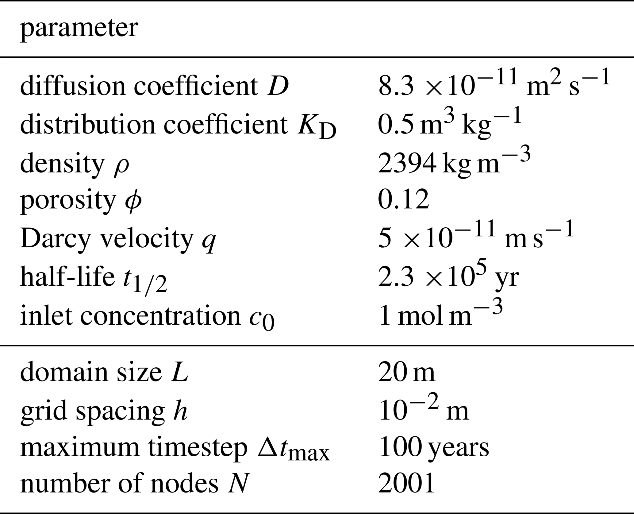
Figure 3 Comparison between the analytic solution by Van Genuchten (1981) (lines) and TransPyREnd (circles) for various times.

We find a good agreement with the analytic solution: The root mean square error (RMSE) is $\mathrm{6}\times {\mathrm{10}}^{-\mathrm{5}}$ mol m⁻³. The total run time is about 17 s on a normal desktop machine. Note that the analytical solution is derived under the assumption of a semi-infinite domain, with the concentration gradient vanishing at infinity. Since we cannot exactly reproduce this boundary condition in a finite domain, we instead chose a no-flow boundary condition on the right edge and made the domain considerably larger than the region where we compare with the analytic solution.

In Fig. 4, we show how the RMSE changes when varying both the time step size Δt and the grid spacing Δx. In the left panel, we vary the grid spacing and keep the time step size fixed, while in the right panel we vary the time step size and keep the grid spacing constant. In general, both methods perform similarly well for reasonable parameter choices. The advantage of the operator splitting, namely allowing for time step sizes larger than the half-life of the relevant nuclide, is not in play in this test, as the half-life is very large compared to the timescale for advection and diffusion. As can be seen in the right panel, the error made by treating the processes of diffusion/advection on the one hand and decay on the other hand quickly rises with growing time step size.

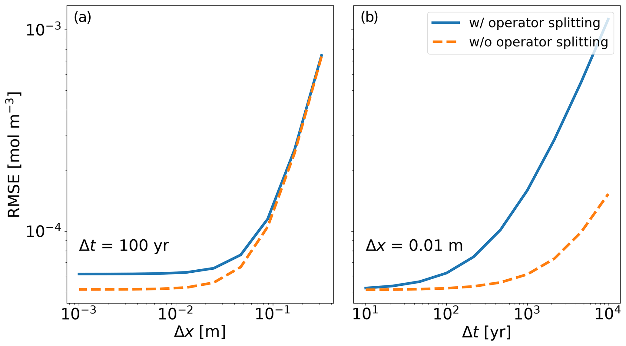
Figure 4 Convergence of the Van Genuchten (1981) test. (a) RMSE as a function of grid spacing. (b) RMSE as a function of time step size.

3.2 Testing Decay Chains

Secondly, we show a test involving both the radioactive decay in a decay chain and diffusion to test the mass conservation of our scheme. We arbitrarily place 1 mol of Cm-245 in the center of a domain with a total length of 1000 m and let the system evolve under decay and diffusion for 10⁶ years. The boundaries are held fixed at a concentration of 0 mol m⁻³. All species in the chain have the same effective diffusion coefficient of 10⁻¹² m² s⁻¹, the porosity is 0.05. The spatial resolution for this test is 1 m. We use the simplified Neptunium chain from Larue et al. (2013) here; the chain and the half-lifes are shown in Table 3, and show results both with and without operator splitting.

Table 3 The simplified Neptunium chain from Larue et al. (2013).

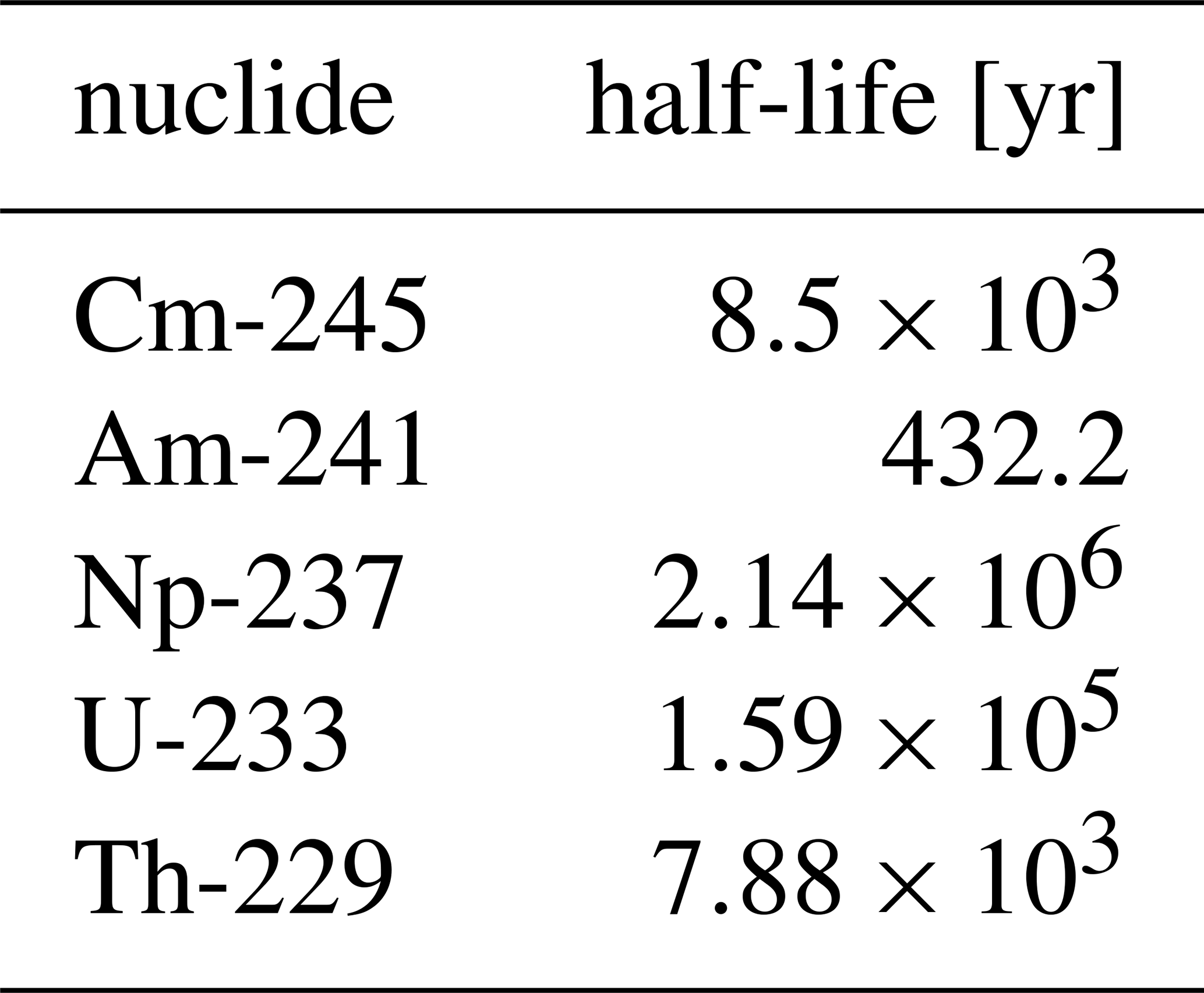
Figure 5 shows the total amount of each of the chain members, that is, the concentration summed over the spatial domain, compared with the solution to the pure decay problem as calculated with the Python package radioactivedecay (Malins and Lemoine, 2022). Again, we are in good agreement, with an RMSE of $\mathrm{2}\times {\mathrm{10}}^{-\mathrm{6}}$ mol m⁻³ both for the run with operator splitting and $\mathrm{5}\times {\mathrm{10}}^{-\mathrm{4}}$ mol m⁻³ for the run without. The execution times differ as well: with operator splitting, the test takes about 4 s on a Desktop machine. Without operator splitting, the test takes about 10 s, due to the stronger constraint on the timestep. In this specific case, we use a timestep of 1000 years for the operator splitting case, and 216 years for the case without operator splitting. We also show a run without the operator splitting scheme for which we enforced a time step of 1000 years. In this case, the RMSE increases to 10⁻² mol m⁻³. The deviations in the short-lived radionuclides become visible towards the end of the simulation time.

Figure 5 Comparison of a simplified nuclide chain (Actinium chain) between radioactivedecay and TransPyREnd. While radioactivedecay (Malins and Lemoine, 2022) solves the pure decay problem, TransPyREnd was run with a simple diffusion+decay setup. In order to compare the two in terms of the conservation of amount of substance, the TransPyREnd concentrations were integrated over the domain to yield the total amount per species. Results are shown with and without operator splitting.

Naturally, the performance gain grows as the minimum half-life in the problem goes down. For example, for the Actinium decay chain, the allowed time step is of the order of 10 years, resulting in a runtime of 36 s without operator splitting, and 4 s with operator splitting. Enforcing the same time step as before will render the system unstable in this case. Thus, depending on the details of the decay chains in question, the operator splitting scheme can provide a relevant improvement in performance.

4 Conclusions and Outlook

In this paper, we have presented the radionuclide transport code TransPyREnd, developed specifically for application in the representative preliminary safety assessments of the German site selection procedure for high-level radioactive waste. The 1D model includes the processes diffusion, advection, sorption, and radioactive decay in the geological barrier. For the model we use a nuclide scheme (Larue et al., 2013) from the literature, pending updates from current BGE research projects. We have summarized the mathematical description of the model, the discretization steps required and our strategy to solve the equations numerically. The code is undergoing rigorous testing and comparison e.g. to OpenGeoSys (Bilke et al., 2022). The benchmarks will be part of a forthcoming paper. TransPyREnd will be made public under an Open-Source license for the community and the interested public in early 2023.

As noted in Sect. 1.1, we have reduced the complexity of the problem by neglecting, in particular, hydraulic, geochemical, mechanical, and thermal processes as well as their coupling. As an example for the possible effect of these additional coupled processes, consider the heating from high-level radioactive waste in the first few hundred years, peaking at up to a few kW per fuel element. The heating has a potential effect on the mechanical state of the deposit and its surroundings (due to thermal expansion) which in turn can affect e.g. the fluid pressure and the porosity of the host rock layer. Both parameters affect the migration of radionuclides.

Our current approach of neglecting these effects is justified by the degree of knowledge about the parameters governing these processes at the current stage of the site selection procedure. However, it is clear that in later stages, these processes need to be carefully addressed to assess their importance to radionuclide migration.

Also, the one-dimensional approach might become less appropriate at later stages, in particular to assess effects arising from complex geometries. While the latter is generally not expected to lead to an increased discharge of radionuclides in the model, the former might have effects in both directions, lowering or enhancing the release of radionuclides in the geosphere/biosphere. At the current stage, the arising uncertainties (i.e. Bjorge et al., 2022) could be considered by systematically varying the model parameters, in particular the diffusion and sorption coefficients. Apart from these considerations, it should be noted that decay processes could also be solved in a semi-implicit fashion by taking advantage of the simple, linear decay chains in our nuclide scheme. The performance of the code could be be imprived by the implementation of a more specialized solving method like the Thomas algorithm (Thomas, 1949). We leave this to future work. Additionally, a near-field model which could consider for instance retention by backfill material is planned for the future.

In the next phases of the site-selection procedure more complex 3D numerical models will be computed. For this aim the OpenWorkFlow project was initiated by BGE (e.g. see https://www.ufz.de/index.php?en=48378, last access: 13 January 2023).