 | 10 Jan 2023
Inverse flow zone characterization using distributed temperature sensing in a deep geothermal production well located in the Southern German Molasse Basin
Felix Schölderle
Daniela Pfrang
Kai Zosseder
The localization and characterization of hydraulically active zones in a geothermal well is a major task in understanding the hydro geothermal reservoir. This is often done based on interpretations of spinner flow meter measurements that are performed at the end of the well test while injecting cold water. Once a production well is equipped with an electric submersible pump, data collection inside the reservoir and monitoring of the flow zones is usually barely possible. In a 3.7 km (MD) deep geothermal production well in Munich, Germany, it was successfully demonstrated in 2019 that a permanently installed optical fiber cable could close this measurement gap. We used this fiber-optic monitoring system to collect distributed temperature data once the well was set into production. We inversely modeled the inflow from the formation into the borehole from the production temperature data with an energy and mass balance model. The derived flow profile correlates with previous flow meter analysis and indicates that a karstified region at the very top of the reservoir is the driving factor for hydraulics and obtained production temperature. Qualitatively, the two profiles acquired by distributed temperature sensing (DTS) and flow meter are matchable, yet the production inflow profile by DTS logging is more differentiated compared to spinner flow meter logs interpretation during injection.
- Article
(1948 KB) - Full-text XML
- BibTeX
- EndNote


Reservoir characterization is a key for ensuring secure and sustainable usage of geothermal resources. One major task is the localization of productive zones in the reservoir, respectively flow zones inside a well and the quantification of the contribution of the single zones to the produced amount of thermal water. Typically, production logging tools equipped with flow meter spinners are used in geothermal wells to estimate hydraulically active zones during injection of water (Schlumberger, 1997). Additionally, wireline temperature runs can be analyzed for non-linearity indicating potential high permeable zones inside a well (e.g., Lim et al., 2020).
During production, data logging in the reservoir is difficult, as permanent deep monitoring tools are rare and in case the well is a production well and equipped with an electric submersible pump (ESP), the deepest measurement point is usually located directly at the bottom of the pump. Monitoring tools below the ESP are not yet standard, but are feasible, as demonstrated in 2019 in a geothermal production well in Munich, Germany, where a fiber-optic cable was installed along a free hanging sucker rod in the middle of the wellbore (Schölderle et al., 2021). This cable enables seismic campaigns via distributed acoustic sensing (DAS) technology, temperature monitoring via distributed temperature sensing (DTS) and measuring point pressure and temperature () at a gauge spliced into the cable on top of the reservoir. Due to its high spatial and temporal resolution, DTS technology, often via cemented cable or wireline designs, has become increasingly popular in geothermal applications in recent years, for both monitoring wellbore stability (e.g., Reinsch, 2012) and reservoir characterization (e.g., Sakaguchi and Matsushima, 2000). Wellbore temperature, respectively heat can be used as a tracer for flow in porous and/or karstified and/or fractured aquifers. With the knowledge of the thermal properties of the reservoir rock and pressure conditions, a flow profile can be back calculated from the temperature data. This was shown by e.g., Pouladiborj (2021) who used the classical approach of energy balance for a control volume inside the producing well of Ramey (1962) and Hasan and Kabir (2010) to inversely derive flow profiles of DTS data of a well in Brittany, France. In addition, there are commercial solutions that allow production profiling by calculating a flow profile from DTS data based on a coupled energy and mass balance model, such as the production log analysis software KAPPA Emeraude (Kotlar et al., 2021), which is widely used in the oil and gas industry.
During the first operation of the monitored well, the installed DTS system provided real-time monitoring in the reservoir and generated flowing temperature data that can be studied inversely to characterize the inflow zones of the reservoir. These results were compared with conventional flow meter interpretations carried out at a time when the ESP was not yet installed to analyze if contributions of the flow zones derived at injection conditions are equivalent to production conditions.
One of Europe's most important low-enthalpy geothermal regions is the Bavarian Molasse Basin in Germany, a north alpine foreland basin spreading between the Swabian and Franconian Alb near the river Danube and the northern alpine front (Meyer and Schmidt-Kaler, 1990). Here, the main target for hydrogeothermal exploration are the Upper Jurassic “Malm” carbonates, which lay in shallow depths in the North and are dipping to the South where they can be found in depths of 4000–6000 m near the northern alpine front (Flechtner et al., 2020). These sedimentary layers partly show high porosities with up to 27.5 % (Zosseder et al., 2022) and high permeabilities (for matrix permeability, core measurements range between 10−4 to 102 mD, Bohnsack et al., 2020), but also high heterogeneity on small regional scales. The production temperatures range between under 40 ∘C in the north and over 160 ∘C in the south (Weber et al., 2019).
The largest geothermal wellsite in the Bavarian Molasse Basin is the “Schäftlarnstraße” (SLS) site in Munich, where six wells were drilled from 2018 to 2020 to depths of approximately 2400 to 3100 m TVD. Three producer wells and three injector wells transverse the stratigraphic layers of Purbeck and Upper Jurassic at different depths, separated by two major faults (see Fig. 1).
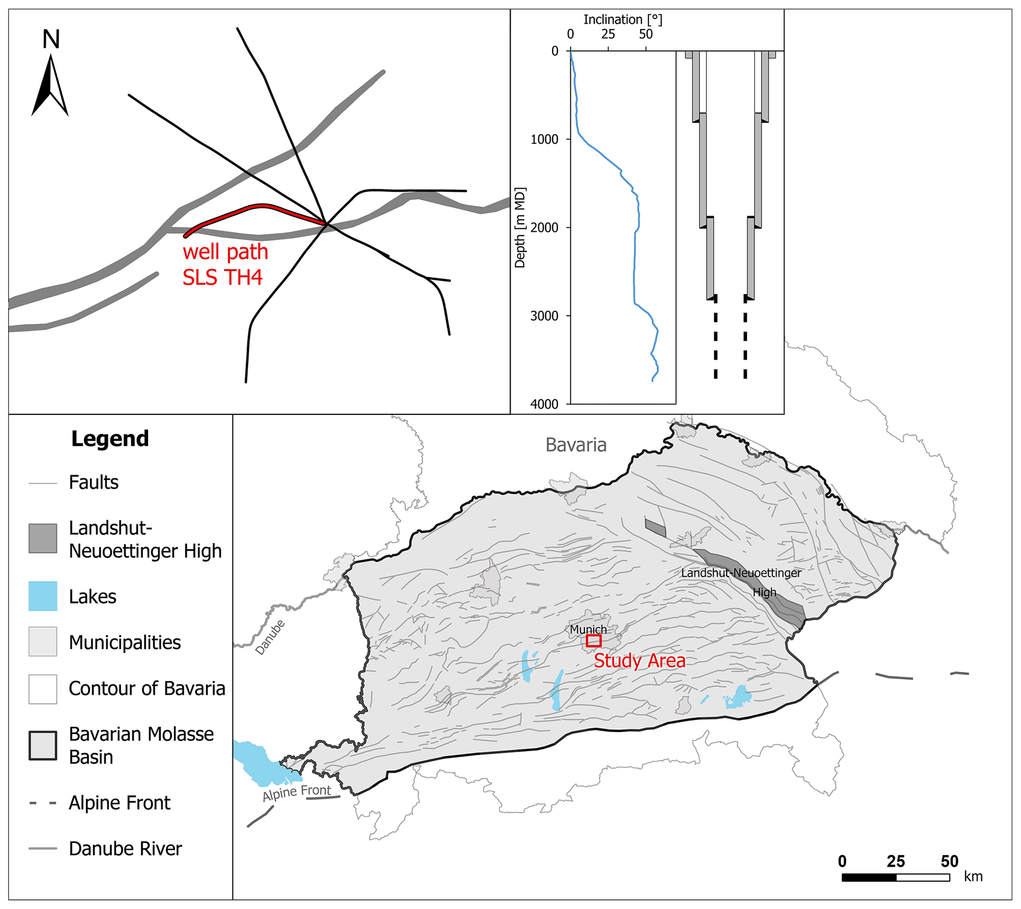
Figure 1Map of the Bavarian Molasse Basin, cropped to Bavaria, and the six well paths at the geothermal study site Schäftlarnstraße with inclination and scheme of well completion of SLS TH4.
Consequently, the highest production temperatures are at the southern and deepest wells with around 105 ∘C. Our studied well is the well SLS TH4 that explores the reservoir to the west. The well is 3.7 km (MD) deep (around 2.9 km TVD) and completed with a perforated liner in the reservoir section. In summer 2019, a spinner flow meter log was recorded over the reservoir in the well SLS TH4 to observe the hydraulic active zones of the well during injection conditions. In November/December 2019, this production well was equipped with a permanent fiber-optic cable, allowing for gathering distributed acoustic and distributed temperature data, as well as point pressure and temperature ( gauge) data at top of the reservoir. The cable was first installed from the wellhead down to a depth of 3690 m MD (2918 m TVD), hanging freely along a sucker-rod construction below a crossover mounted to the liner hanger. Two months after installation, DTS data were collected during two cold-water injection tests in January and February 2020 to verify the flow meter interpretation. The results and further details about the installation were discussed in Schölderle et al. (2021) and indicated that a small karstified region (25 m thick) directly at the top of the reservoir is the dominant hydraulically active zone of the well. It was supposed that less than 8 % of flow contributes from regions deeper in the well. When the ESP was installed in April 2021, the free-hanging sucker-rod construction was installed below the pump at 760 m depth to a total depth of 3684 m MD (2914 m TVD). Above the pump, the cable was routed outside the production tubing to the wellhead. After further 16 months of shut-in time, the well was set into production for the first time in summer 2021.
We used the fiber-optic monitoring system at the geothermal site “Schäftlarnstraße” to collect DTS data during the start of production. At this production period, two of the three doublets at the study site were simultaneously producing.
An energy balance model was used to inversely derive a production flow profile from the DTS profiles of the SLS TH4 well using the software KAPPA Emeraude (v5.40). Reservoir pressure and geothermal gradient are two required model inputs, which we estimated from the fiber optic system. The thermal gradient inside the reservoir was evaluated based on a series of DTS profiles measured over one year of the shut-in period. The pressure could be derived from the fiber-optic gauge located at top of the reservoir.
3.1 Fiber-optic data at the well SLS TH4
Fiber-optic temperature data has been collected continuously since the installation of the system in November/December 2019, except for two major interruptions in the spring of 2020 when the measurements had to be stopped due to surface installation work, and in April 2021, when the monitoring system was modified during ESP installation (see Fig. 2).

We acquired DTS profiles every 10 min at a spatial sampling of 0.25 m and processed the data by averaging over a window of 6 h and spatial resolution of 1 m. The resulting temperature resolution of the profiles is about 0.13 K.
To derive the geothermal gradient in the reservoir, we studied the profiles collected immediately before the start of production, as in the early stage of geothermal wells, borehole temperature logs reflect the geothermal gradient insufficient because the near surrounding of the well is often still thermally affected by the preceding drilling or testing works (e.g., Eppelbaum et al., 2014). Figure 3a shows the heating of the borehole after drilling and testing based on a series of DTS profiles averaged over 6 h from the period between the cold-water injection tests in winter 2020 and the start of production in summer 2021.

Figure 3(a) DTS profiles between July 2020 and July 2021 and a schematic of the wellbore with sketched fiber-optic cable (yellow line) clamped to sucker rod (grey line) and (b) temperatures at different depths plotted versus time. The grey DTS profiles in (a) are from the shut-in period before the ESP was installed and the blue DTS profiles were measured after installation. The displayed DTS data are averaged over 6 h at a spatial resolution of 1 m. The temperature anomaly below 2750 m in (a) is a measuring fragment due to the inline splice from the downhole gauge.
The segment presented in Fig. 3a shows a part of the cased 12.25-inch section and the upper 250 m of the reservoir section, where we can see a non-linear anomaly in the profiles compared to the remaining more uniform trend. At stable conditions, changes in the slope of temperature profiles can imply groundwater flow in up- or downwards direction (e.g., Lim et al., 2020). Since we can still see a dynamic behavior at the thermal anomaly, stable conditions are not met in this region. From Fig. 3b, it becomes clear that the region between 2800 and 2950 m MD was still warming up, while the sections above and below the anomaly seem to be thermally fully equilibrated. To estimate the geothermal gradient, we therefore extrapolated over the anomaly, starting from the stable DTS profiles deeper in the reservoir.
3.2 Inverse flow profiling from DTS data
We used the commercial well interpretation software KAPPA Emeraude (v5.40) to calculate a flow profile from the collected DTS production data. The underlying physical equations are based on the works of Pucknell and Clifford (1991), Chen et al. (1995) and Hasan and Kabir (2002) and their integration into the Emeraude energy model was described by Kotlar et al. (2021). The used model builds on a coupling of pressure and temperature into an energy balance model for segments of the wellbore and respective volume for the reservoir.
The energy balance for an infinite segment of a producing well in steady-state condition is given as:
with , where qs ((kg s−1) kg−1) is the specific mass rate (mass rate divided by mass), hs (J kg−1) the specific enthalpy, which is dependent on pressure, A (m2) the flow area, ρs ((kg m−3) kg−1) the specific density, g=9.81 (m2 s−1) the gravitational acceleration, dl (m) the length of the respective segment and ΔT (K) the temperature change. D is the thermal conductance term as defined by Kotlar et al. (2021) and its unit is given through its definition as (1 mKs−3). The subscripts in the equation represent b below the segment, a above the segment, s in the segment and sf the sand face (wellbore/reservoir interface). Equation (1) can be read as follows: The convective heat flux out of the segment (term on the left-hand side) equals the convective heat flux into the segment from below (first term on the right-hand side) plus the convective heat flux from the reservoir into the wellbore (second term on the right-hand side) plus the conductive heat flux from the sand face to the well (third term on the right-hand side). The conductive term D bases on Ramey's (1962) approach of calculating a total heat transfer coefficient for the wellbore system. The convective terms include the transport of internal, kinetic and potential energy, e.g., the expansion work dependent on the respective pressure.
For neglected vertical conductive transport, the energy balance for a small volume inside the reservoir in steady state writes as:
with , where the subscript “res” represents the reservoir and Tgeo (∘C) is the geothermal temperature far away from the borehole. The exact deduction of Eqs. (1) and (2) can be reviewed in Kotlar et al. (2021).
The modelling workflow is as follows: We assume that the reservoir fluid far away from the well is at the temperature of the geothermal gradient Tgeo. With knowledge of Tgeo, fluid properties and pressure, Eqs. (1) and (2) can be solved iteratively for the temperature at the interface reservoir/well Tsf and the temperature at the segment Ts until convergence with the measured temperature profile (DTS production profile). At convergence (minimized error between simulated temperature profile and measured DTS profile), a quantitative production profile over the different segments of the well can be generated. Finally, with the known flow rate from the surface (pump rate during production), the flow profile can be evaluated by checking the deviation of the cumulative sum of the flow profile from the known pump rate.
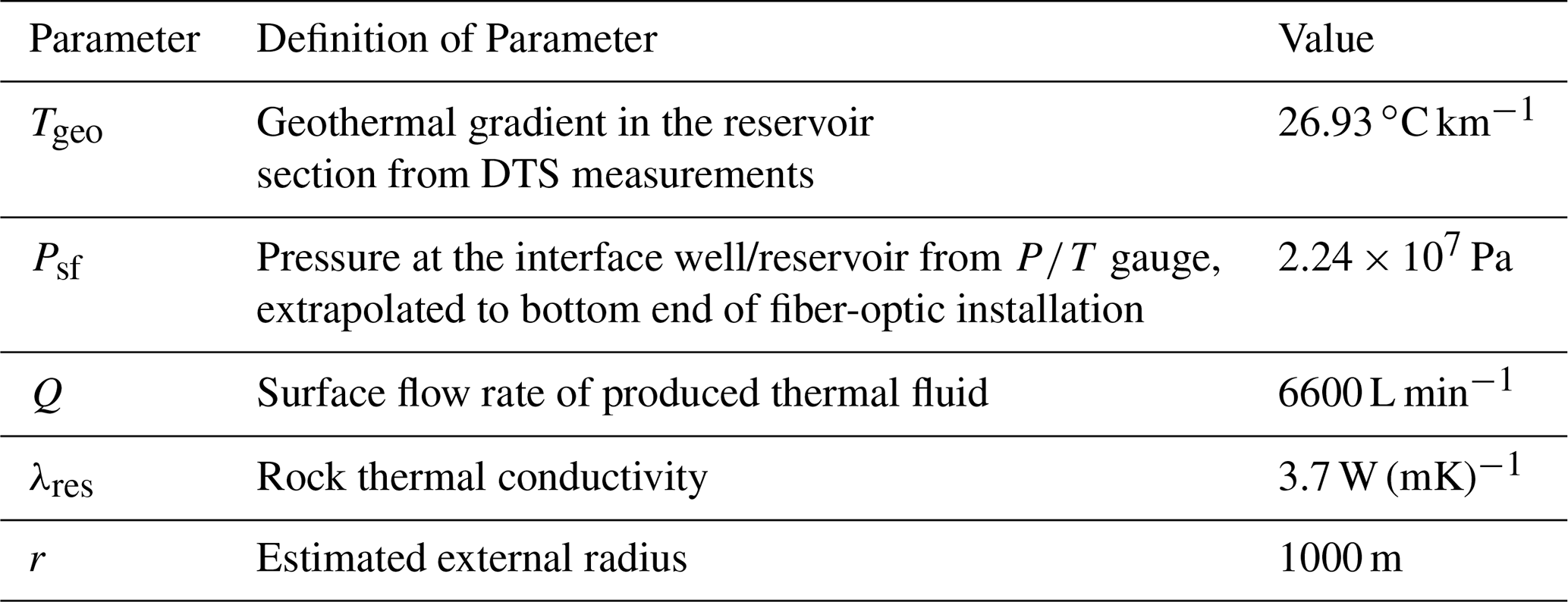
To estimate the geothermal gradient, we used the extrapolated temperature as shown in Fig. 3a. The radius of the reservoir section was taken from open-hole caliper measurements. The sand face pressure was estimated from measured data at the fiber-optic gauge. Equations (1) and (2) include the flow model (mass rates q). Additional required input parameters for the applied production profiling are shown in Table 1.
Table 1Input parameter for the inverse DTS profiling with KAPPA Emeraude.
The model of Kotlar et al. (2021) can either calculate the pressure drop due to frictional loss at the flow zones between the reservoir pressure (pressure at large distance to the well) and sand face pressure from Skin, via porosity and permeability inputs (see Kotlar et al., 2021), or let the user manually define a pressure loss at each segment. Due to the injection profiling, we know that the upper part of the reservoir is a highly hydraulically active zone. A higher friction related pressure loss can therefore expected here due to changing flow velocity:
where Δp (Pa) is the loss of pressure, f (-) is the friction factor, l (m) is the length of the segment, ρ (kg m−3) is the density of the fluid, which was calculated according to the IAPWS-IF97 formulation (Cooper and Dooley, 2007), d (m) is the diameter and v (m s−1) is the flow velocity. During the modelling process we manually assumed the pressure loss until a good fit (minimized error of modelled with measured temperature and pump rate) was achieved.
We used the permanent fiber-optic monitoring system of the well SLS TH4 to gather DTS data during start of production and derived a production flow profile with the inverse model of Kotlar et al. (2021). Figure 4a shows the converged modeled temperature compared to the DTS profile during production and the temperature gradient from extrapolating the undisturbed DTS profiles as shown in Fig. 3a. Figure 4b shows the interpreted inflow as a cumulative profile and contribution per flow zone.
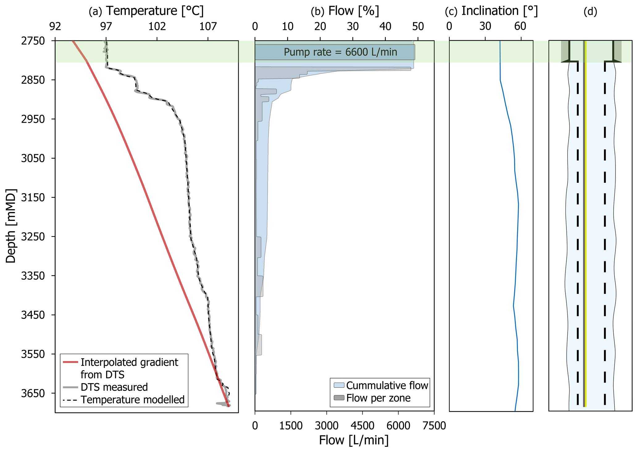
Figure 4Results of DTS production profiling model inside the reservoir of SLS TH4. (a) Measured temperature (DTS, grey line) and modelled temperature (black dashed line) with estimated geothermal gradient (red line) versus depth, (b) modelled contribution of flow (grey) and cummulative flow in the bore (light blue) in comparison to surface pump rate (blue), (c) Inclination of the well, (d) well sketch of reservoir section. The olive band highlights the casing section. The shown results were generated with KAPPA Emeraude (v5.40).
A satisfactory fit with both DTS production profile and surface pump rate was achieved. From the interpreted contributions, we can distinguish four different hydraulically active zones. The most prominent zone is between 2820 and 2855 m MD, for which an inflow participation of 78 % was interpreted. About 14 % flow were calculated at 2875 to 2955 m MD. The calculations show two minor flow zones at 3255 to 3400 m MD and 3455 to 3555 m MD with less than 5 %, respectively 3 % flow.
In Schölderle et al. (2021), more than 90 % of flow were interpreted at injection conditions (spinner flow meter measurements) at a karstified zone at the very top of the reservoir in the stratigraphic layer of the Purbeck. Table 2 shows a comparison of the updated interpretation at production conditions with the flow meter interpreted zone contributions at injection conditions.
Table 2Comparison of flow zones interpreted from DTS production data with flow zone interpretation from flow meter data at injection.
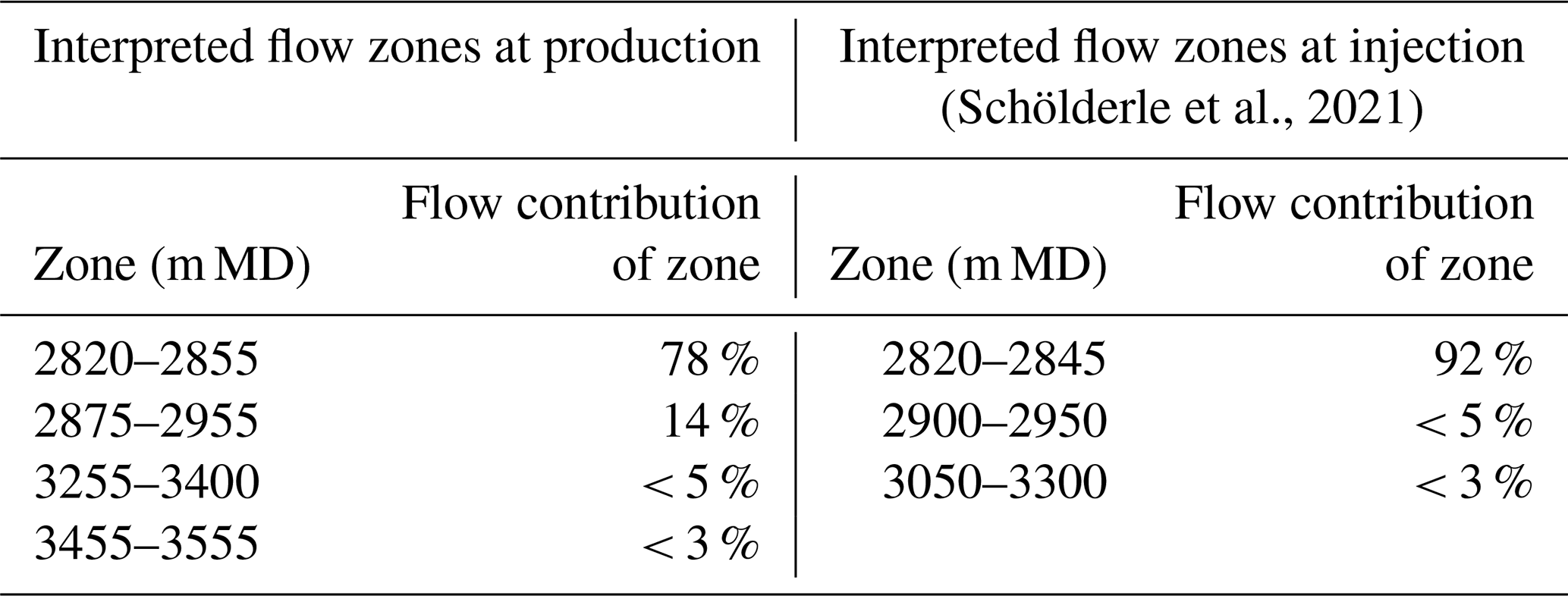
In a qualitative manner, both methods show that the upper 25 m thick (from flow meter interpretation), respectively 35 m thick (from inverse modeling) karstified zone is the dominant hydraulic contributor in the reservoir. However, a higher inflow rate in deeper regions of the reservoir was interpreted from the production DTS data than was previously possible using only flow meter data at injection.
Both methods, flow meter interpretation and inverse DTS production profiling bear some uncertainties. Concerning the spinner flow meter run, we have to consider the high inclination (see Fig. 4c) in the reservoir section and the completion with the perforated liner, which is likely to provoke complicated flow regimes and turbulences, e.g., due to flow behind the liner (Haoua et al., 2015; Zarrouk and McLean, 2019). Furthermore, the quality of flow meter measurements is dependent on a smooth run of the tool (Schlumberger, 1997). In addition, due to the closeness of the hydraulically active zone to the liner hanger, it is likely that the change of the diameter leads to turbulences that might disturb the spinner velocity.
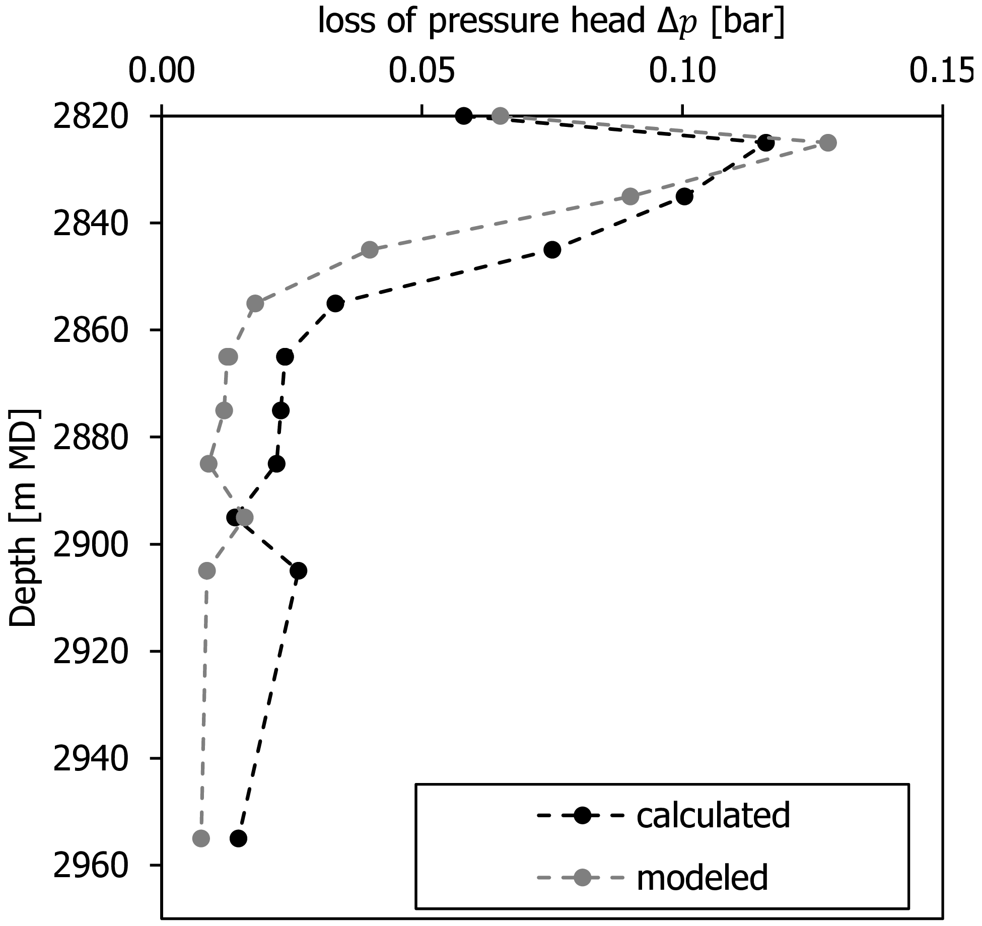
Figure 5Comparison of pressure loss at the main flow zone estimated as input for Emeraude modelling with analytically calculated pressure loss.
The uncertainty of the modelling solution on the other hand is dependent on the models limitations and the errors that lie in the assumed input parameters. As shown in Fig. 3a and b, we had to assume parts of the geothermal gradient as the shut-in DTS profiles were not yet completely equilibrated. Concerning the reservoir pressure, we used the data measured at the gauge during shut-in and during production. The production-profiling module (Emeraude KAPPA, Kotlar et al., 2021) allows for calculating the production pressure profile from user input of skin factor at each flow zone and permeability and porosity. As those values were unknown, we iteratively changed the pressure loss at the zones manually until the model converged. A simple friction pressure loss model can show if the assumed pressure loss beforehand can be calculated from the achieved flow profile. To do so, we calculated the flow velocity from the modelled flow profile with a simplified flow cross-section, taking the drill bit size of the reservoir section (8.5 inch) subtracted with the thickness of the perforated liner and neglecting outbreaks in the rock and the narrowing of the cross-section due to the fiber-optic cable. We took the roughness of the pipe (perforated liner) as m (e.g., Codo et al., 2012) and calculated the friction factor f with the common equations of Nikuradse, Colebrook and White and Blasius (Lipovka and Lipovka, 2014). Following Eq. (3), we then determined the pressure loss at different depths. As shown in Fig. 5, the assumed pressure loss used as input for the model and the calculated pressure loss from the obtained flow profile follow the same trend and are in the same magnitude at the different flow zone depths.
The results presented show that the permanent fiber-optic system can lead to a deeper understanding of the reservoir, which is important to ensure sustainable and secure use of the heat source thermal water. DTS data from production can be used for inverse production profiling as a viable alternative to common injection profiling methods and additionally enable permanent monitoring of any changes and divergences in production. Throughout the acquisition of the presented data, two of the three doublets at the site were running and might have affected each other. Therefore, DTS measurements for inverse production profiling will be continued during the upcoming long-term production tests to evaluate if different configurations (only one active doublet or all three doublets in production) lead to different model solutions.
The code for the inverse model is included in the commercial software KAPPA Emeraude. Please contact the corresponding author for information about the additional code used for the pressure loss model.
Data is available from the corresponding author on reasonable request.
FS performed the analyses and modelling. FS, DP and KZ shaped the research and wrote the manuscript. KZ helped providing funding and revised the manuscript. All authors read and agreed to the published version of the manuscript.
The contact author has declared that none of the authors has any competing interests.
Publisher’s note: Copernicus Publications remains neutral with regard to jurisdictional claims in published maps and institutional affiliations.
This article is part of the special issue “European Geosciences Union General Assembly 2022, EGU Division Energy, Resources & Environment (ERE)”. It is a result of the EGU General Assembly 2022, Vienna, Austria, 23–27 May 2022.
We are grateful for the support of Stadtwerke München SWM, who are the owners of the monitored well and who made the research possible. We would like to especially thank Michael Meinecke for his commitment to the project. We also thank the two anonymous reviewers for their generous time in providing comments and suggestions that helped us to improve the paper.
This research has been supported by the Bundesministerium für Wirtschaft und Energie (grant no. 0324332B) and the Bayerisches Staatsministerium für Wissenschaft und Kunst (grant no. Geothermie-Allianz Bayern).
This work was supported by the German Research Foundation (DFG) and the Technical University of Munich (TUM) in the framework of the Open Access Publishing Program.
This paper was edited by Gregor Giebel and reviewed by two anonymous referees.
Bohnsack, D., Potten, M., Pfrang, D., Wolpert, P., and Zosseder, K.: Porosity–permeability relationship derived from Upper Jurassic carbonate rock cores to assess the regional hydraulic matrix properties of the Malm reservoir in the South German Molasse Basin, Geotherm. Energy, 8, 12, https://doi.org/10.1186/s40517-020-00166-9, 2020.
Chen, G., Tehrani, D. H., and Peden, J. M.: Calculation Of Well Productivity In A Reservoir Simulator (I), SPE-29121-MS, https://doi.org/10.2118/29121-MS, 1995.
Codo, F. P., Adomou, A., and Adanhounmè, V.: Analytical Method for Calculation of Temperature of the Produced Water in Geothermal Wells, Int. J. Sci. Eng. Res., 3, 1–7, 2012.
Cooper, J. R. and Dooley, R. B.: The International Association for the Properties of Water and Steam, 1–49, Lucerne, Switzerland, http://www.iapws.org/relguide/IF97-Rev.pdf (last access: 1 June 2022), 2007.
Eppelbaum, L., Kutasov, I., and Pilchin, A.: Applied Geothermics, Springer Berlin Heidelberg, https://doi.org/10.1016/0160-9327(87)90297-3, 2014.
Flechtner, F., Loewer, M., and Keim, M.: Updated stock take of the deep geothermal projects in Bavaria, Germany (2019), in: Proceedings World Geothermal Congress 2020 Reykjavik, Iceland, 26 April–2 May 2020 Updated, 2020.
Haoua, T. Ben, Abubakr, S., Pazzi, J., Djessas, L., Ali, A. M., Ayyad, H. B., and Boumali, A.: Combining Horizontal Production Logging and Distributed Temperature Interpretations to Diagnose Annular Flow in Slotted-Liner Completions, 1–13, https://doi.org/10.2118/172593-MS, 2015.
Hasan, A. and Kabir, S.: Modeling Two-Phase Fluid and Heat Flows in Geothermal Wells, J. Petrol. Sci. Eng., 71, 77–86, https://doi.org/10.1016/j.petrol.2010.01.008, 2010.
Hasan, A. R. and Kabir, C. S.: Fluid flow and heat transfer in wellbores, Society of Petroleum Engineers, ISBN 978-1-55563-094-2, 175 pp., 2002.
Kotlar, N., Allain, O., Benano, L., and Artus, V.: Cased Hole Logging v5.40 The theory and practise of cased hole log acquisition and analysis and their application to well integrity, production profiling and reservoir monitoring, 366 pp., https://www.kappaeng.com/downloads (last access: 1 June 2022), 2021.
Lim, W. R., Hamm, S. Y., Lee, C., Hwang, S., Park, I. H., and Kim, H. C.: Characteristics of deep groundwater flow and temperature in the tertiary Pohang area, South Korea, Appl. Sci., 10, 1–21, https://doi.org/10.3390/app10155120, 2020.
Lipovka, A. Y. and Lipovka, Y. L.: Determining hydraulic friction factor for pipeline systems, Journal of Siberian Federal University, Eng. Technol., 7, 62–82, http://elib.sfu-kras.ru/handle/2311/10293 (last access: 1 June 2022), 2014.
Meyer, R. K. F. and Schmidt-Kaler, H.: Paläogeographie und Schwammriffentwicklung des süddeutschen Malm- ein Überblick [Paleogeography and Development of Sponge Reefs in the Upper Jurassic of Southern Germany – An Overview], Facies, 23, 175–184, https://doi.org/10.1007/BF02536712, 1990.
Pouladiborj, B.: The use of heat for subsurface flow quantification and understanding the subsurface heterogeneity, Université Rennes, https://ged.univ-rennes1.fr/nuxeo/site/esupversions/da77a25d-ef8a-45dc-aca7-7d3c62c29537?inline (last access: 1 June 2022), 2021.
Pucknell, J. K. and Clifford, P. J.: Calculation of Total Skin Factors, Paper presented at the SPE Offshore Europe, Aberdeen, United Kingdom, https://doi.org/10.2118/23100-MS, 1991.
Ramey Jr., H. J.: Wellbore Heat Transmission, J. Petrol. Technol., 14, 427–435, https://doi.org/10.2118/96-PA, 1962.
Reinsch, T.: Structural integrity monitoring in a hot geothermal well using fibre optic distributed temperature sensing, Clausthal University of Technology, 243 pp., http://nbn-resolving.de/urn/resolver.pl?urn=urn:nbn:de:gbv:104-1111221 (last access: 1 June 2022), 2012.
Sakaguchi, K. and Matsushima, N.: Temperature Logging By the Distributed Temperature Sensing, in: Proceedings World Geothermal Congress 2000, Kyushu – Tohoku, Japan, 28 May–10 June 2000, 1657–1661, https://www.geothermal-energy.org/pdf/IGAstandard/WGC/2000/R0400.PDF (last access: 1 June 2022), 2000.
Schlumberger: Cased Hole Log Interpretation Principles/Applications, 4th Edn., Schlumberger, Pennsylvania State University, 212 pp., document no. SMP-7025, 1997.
Schölderle, F., Lipus, M., Pfrang, D., Reinsch, T., Haberer, S., Einsiedl, F., and Zosseder, K.: Monitoring cold water injections for reservoir characterization using a permanent fiber optic installation in a geothermal production well in the Southern German Molasse Basin, Springer Berlin Heidelberg, https://doi.org/10.1186/s40517-021-00204-0, 36 pp., 2021.
Weber, J., Born, H., and Moeck, I.: Geothermal Energy Use, Country Update for Germany 2016–2018, in: European Geothermal Congress 2019, Den Haag, The Netherlands, 11–14 June, 2019.
Zarrouk, S. J. and McLean, K.: Geothermal Well Test Analysis Fundamentals, Applications and Advanced Techniques, Elsevier, ISBN 978-0-12-819266-5, 226 pp., 2019.
Zosseder, K., Pfrang, D., Schölderle, F., Bohnsack, D., and Konrad, F.: Characterisation of the Upper Jurassic geothermal reservoir in the South German Molasse Basin as basis for a potential assessment to foster the geothermal installation development – Results from the joint research project Geothermal Alliance Bavaria, Geomech. Tunnell., 15, 17–24, https://doi.org/10.1002/geot.202100087, 2022.