Strength and Challenges of global model MPAS with regional mesh refinement for mid-latitude storm forecasting: a case study

With the rising share of renewable energy sources like wind energy in the energy mix, high-impact weather events like mid-latitude storms increasingly affect energy production, grid stability and safety and reliable forecasting becomes very relevant for e.g. transmission system operators to allow for actions to reduce imbalances. Traditionally, meteorological forecasts are provided by limited-area weather prediction models (LAMs), which can use high enough model resolution to represent the range of atmospheric scales of motions associated with such storm structures. While generally satisfactory, deterioration and insufficient deepening of large-scale storm structures are observed when they are introduced near the lateral boundaries of the LAM due to inadequate spatial and temporal interpolation. Global models with regional mesh refinement capabilities like the Model for Prediction Across Scales (MPAS) have the potential to provide an alternative, while avoiding sharp resolution jumps and lateral boundaries. In this study, MPAS' capabilities of simulating key evaluation metrics like storm intensity, storm location and storm duration are investigated based on a case study and assessed in comparison with buoy measurements, forecast products from the Climate Forecast System (CFSv2) and simulations with the Weather Research and Forecasting (WRF) LAM. Quasi-uniform and variable-resolution MPAS mesh configurations with different model physics settings are designed to analyze the impact of the mesh refinement and model physics on the model performance. MPAS shows good performance in predicting storm intensity based on the local minimum sea level pressure, while time of local minimum sea level pressure (storm duration) was generally estimated too late (too long) in comparison with the buoy measurements in part due to an early west-wards shift of the storm center in MPAS. The variable-resolution configurations showed a combination of an additional south-westwards shift and deviations in the sea level pressure field south-west of the storm center that introduced additional bias to the time of local minimum sea level pressure at some locations. The study highlights the need for a more detailed analysis of applied mesh refinements for particular applications and emphasizes the importance of methods like data assimilation techniques to prevent model drifts.

1 Introduction

Within the field of wind energy, weather patterns like mid-latitude cyclones can affect several aspects of wind power production. The associated weather conditions characterized by wind gusts and high near-surface winds (Collier et al., 1994; Browning, 2004) can amplify wind energy production, but can also impose additional stress on the electrical grid, or, in the worst case, cause physical damage to infrastructure. Especially the frontal systems that are tightly connected with the passing low pressure system can cause sharp ramps in the power production (Steiner et al., 2017) or shut-down of whole wind farms when cut-out wind speed criteria are exceeded (Cutululis et al., 2012). This affects, among others, grid stability and safety (Cutululis et al., 2012; Steiner et al., 2017) and can also affect the energy market (Artipoli and Durante, 2014). Regions like the North Sea, where weather is primarily guided by mid-latitude cyclones (Catto et al., 2019) and the spatial concentration of installed wind power capacity is high (e.g. WindEurope, 2020), are especially vulnerable to this. Steiner et al. (2017) found that about 38 % of day-ahead wind power forecast errors between 2012 and 2014 in Germany were connected to extra-tropical cyclones located over the North Sea, Germany or the Baltic Sea. Highly reliable forecasts of mid-latitude cyclones are, therefore, seen as a crucial element to allow adequate responses and proper storm management (Cutululis et al., 2011), but they are also very challenging for weather prediction models to obtain (e.g. Jung et al., 2004; Doyle et al., 2014). From a modeling perspective, origins in mid-latitude storm forecast errors can be various (sensitivity to initial conditions, e.g. Zou et al., 1998 or model physics, e.g. Pradhan et al., 2018), but one important factor commonly observed in limited-area models (LAM) is connected with the impact of lateral boundary conditions on storm development (Gustafsson, 1990; Gustafsson et al., 1998; Termonia, 2003; Termonia et al., 2009; Imberger et al., 2020). Especially when the large-scale storm structures need to be introduced from the external forcing data into the LAM, temporal and spatial interpolation can result in insufficient representation of storm intensity (Termonia, 2003; Termonia et al., 2009) and storm displacements (Imberger et al., 2020). Based on a case study of storm Christian (October 2013, Hewson et al., 2014), Imberger et al. (2020) investigated an especially critical situation where a large-scale storm feature is introduced at a lateral boundary corner of the Weather Research and Forecasting (WRF, Skamarock et al., 2008) model. The misinterpretation due to spatial and temporal interpolation resulted in a lack of storm deepening and displacement of the storm structure. This issue is further referred to as “corner issue”. While more frequent update intervals of the LBCs were shown to improve the forecast (Imberger et al., 2020), the inherent challenges with the LBCs and critical LAM corner regions remain. In this investigation, an alternative approach to the limited-area model is investigated, which makes use of the global Model for Prediction Across Scales (MPAS, Skamarock et al., 2012). Its mesh discretization (Spherical Centroidal Voronoi Tessellation, SCVT, Du et al., 1999, 2003) allows the design of globe-spanning meshes with smooth transition to regional refinement regions (Ringler et al., 2010), thus avoiding the challenges with LBCs, sudden resolution jumps and effects like the previously mentioned “corner issue” as investigated in Imberger et al. (2020). MPAS has already been applied in a range of applications, among others, for the investigation of the extratropical transition of tropical cyclones, (Michaelis et al., 2019; Michaelis and Lackmann, 2019), wind speed variability during open cellular convection (Imberger et al., 2021) and forecasting of extreme weather events over Europe (Kramer et al., 2020). While potential benefits are visible, it is not straight-forward to determine whether, where and to what degree they also translate to case specific applications like mid-latitude storm forecasting. Motivated by the challenges (poor representation of storm deepening and location as a result of spatial and temporal interpolation effects at the LAM boundaries) observed in Imberger et al. (2020), storm Christian has been selected as a case study to further investigate MPAS' potential for mid-latitude forecasting applications. A combination of a quasi-uniform 54 km and a variable 54–18 km mesh with different model physics configurations have been tested and analyzed against buoy measurements, WRF model results from Imberger et al. (2020) and Climate Forecast System (CFSv2, Saha et al., 2011) 6-hourly forecasts to assess whether and where MPAS can enhance the forecasting of key storm metrics and what impact the mesh refinement and choice of model physics have. Section 2 provides an overview of the methodology and data sets used including a definition of the key evaluation metrics (storm intensity, time of local minimum sea level pressure as a measure of storm location and storm duration), the buoy observations and the WRF and MPAS setup and model data. Results and discussion are presented in Sects. 3 and 4, respectively. Conclusions are presented in Sect. 5.

2 Methods

2.1 Evaluation metrics

To evaluate the forecast capabilities of the models, three evaluation metrics have been defined: storm intensity, time of local minimum sea level pressure (t_LMSLP) as an indicator for storm location and storm duration, which are defined in Fig. 1. These metrics are derived from the sea level pressure time-series, which is commonly used to identify storm intensity (in the form of magnitude of minimum sea level pressure) and location (e.g. Grieger et al., 2018). While the chosen metrics are relatively simple, the simplicity allows point measurements, like buoys, to be used for supporting model validation and comparison. At the same time, the metrics contain enough information about the position and strength of the storm structure to evaluate and compare key strengths and weaknesses of the model performance like phase shifts.

Figure 1 Definition of the three evaluation metrics storm intensity (1), time of local minimum sea level pressure t_LMSLP (2) and storm duration (3) derived from the local minimum sea level pressure (LMSLP) and pressure threshold p_t = LMSLP + 10 hPa.

2.2 Buoy measurements

Sea level pressure time series with hourly temporal resolution from six buoy locations are used to validate and compare the simulation results with respect to the evaluation metrics mentioned in Sect. 2.1. Their locations are depicted in Fig. 2, and key information (name, geographic location) is summarized in Table 1. Table 1 also states the sea level pressure threshold p_t used for the storm duration metric at each of the stations. Due to the weak imprint of storm Christian at station #12, it is not included in the storm duration analysis. The buoy data is obtained from the European Marine Observation and Data Network (EMODnet) – Physics System (Novellino et al., 2015).

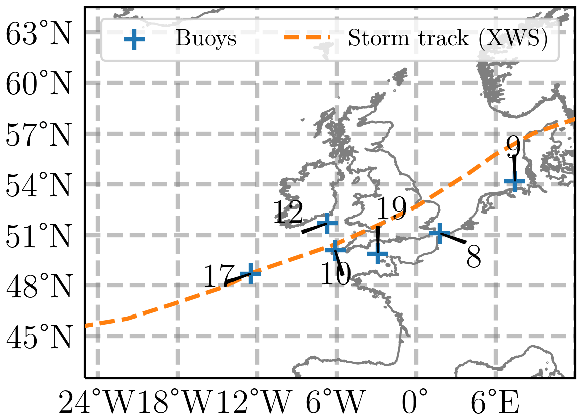
Figure 2 Geographic location of the six buoys together with the track of storm Christian obtained from the Extreme Wind Storms Catalogue (XWS, Roberts et al., 2014, http://www.europeanwindstorms.org, last accessed: 21 October 2021) for reference.

Table 1 Identifiers, geographic location of the six buoy locations as well as the sea level pressure threshold p_t used for the storm duration analysis at that station. Stations are listed from west to east.

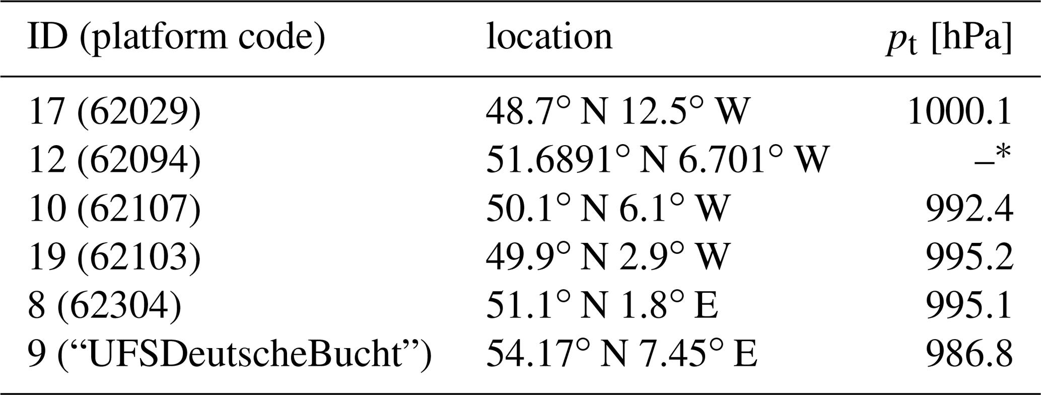
^* Not included in storm duration analysis.

2.3 Extended WRF Simulations from Imberger et al. (2020)

The seven WRF configurations introduced in Imberger et al. (2020) have been adapted for this investigation to allow for comparison between WRF and MPAS, by extending the total simulation time from 36 to 72 h to cover the full period of interest in this work. A short description of the main characteristics of the different WRF configurations, and a depiction of the two different limited-area domains is given in Table 2 and Fig. 3, respectively. All WRF configurations are using a single domain of 18 km grid spacing and have been initialized at 26 October 2013, 12:00 UTC from the 0.5^∘ × 0.5^∘ CFSv2 6-hourly forecast product. The CFSv2 data set provides also the lateral boundary conditions for the WRF runs and the sea level pressure field provided by CFSv2 is also been used in addition to the observational buoy data set for comparison with the other models. For a more extensive description of the WRF configurations, model physics etc., the reader is kindly referred to Imberger et al. (2020).

Table 2 Summary table of the seven WRF configurations with their identifier and a short description of their characteristics. Table adapted with modifications from Imberger et al. (2020), Table 2.

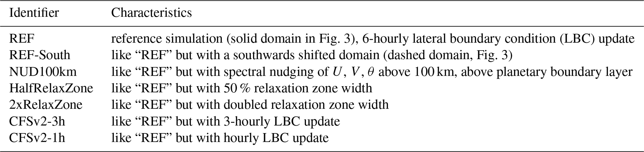
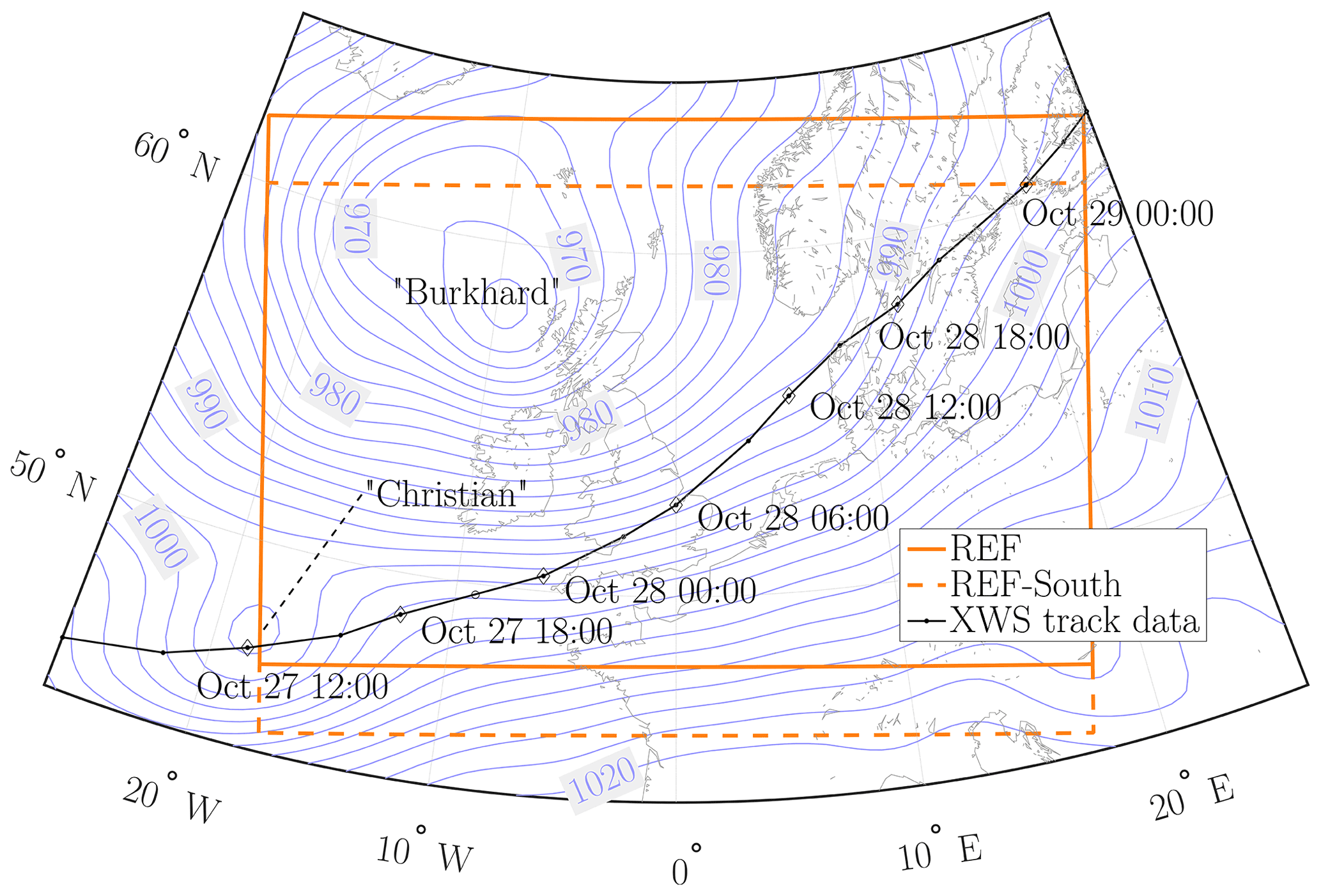
Figure 3 Depiction of the WRF domains “REF” and “REF-South” used in the analysis in Imberger et al. (2020) together with the contour of sea level pressure of CFSv2 at 27 October 2013, 12:00 UTC showing the location of storm Christian and low Burkhard. The storm track from the Extreme Wind Storms Catalogue is included as well. Reprinted from Imberger et al. (2020), copyright 2020 Royal Meteorological Society.

2.4 MPAS Model Setup

Figure 4a depicts the Voronoi cell size distribution of the two mesh configurations in this work: A quasi-uniform 54 km mesh configuration with 204 802 Voronoi cells (further referred to as X1 configuration) and a 54 km mesh configuration with a circular refinement region with 18 km grid spacing (variable-resolution mesh, 245 762 Voronoi cells, further referred to as X3). An overview of the distribution of grid cell spacing in X1 and X3 is given in Fig. 4a. The refinement zone grid spacing and its location in X3 has been inspired by the 18 km grid spacing and placement of WRFs “REF” domain (beginning of the transition zone coincides with REF's south–west corner, where the storm center enters the domain, Fig. 4b). The outermost grid spacing has been chosen to be similar to the 0.5^∘ × 0.5^∘ grid spacing of the CFSv2 forecast product that is used for model initialization (same for the WRF configurations). The impact of different physics settings was investigated by running each mesh configuration using three different physics configurations: The two MPAS default physics suites “convection_permitting” (further refered to as “CP”) and “mesoscale_reference” (“MESO”), as well as, a modified version of “CP” that resembles the combination of physics used in the WRF configurations (“CPKF”). In CPKF, the default cumulus parameterization scheme (scale–aware Grell–Freitas, Grell and Freitas, 2014) has been replaced by the Kain–Fritsch scheme (Kain, 2004). A summary of the six MPAS model configurations is provided in Table 3. The time steps for the two mesh configurations are uniform over the whole mesh and have been adapted to the smallest grid distances to guarantee model stability. This results in a time step of 300 s for the X1 mesh configurations and 100 s for the X3 mesh configurations.

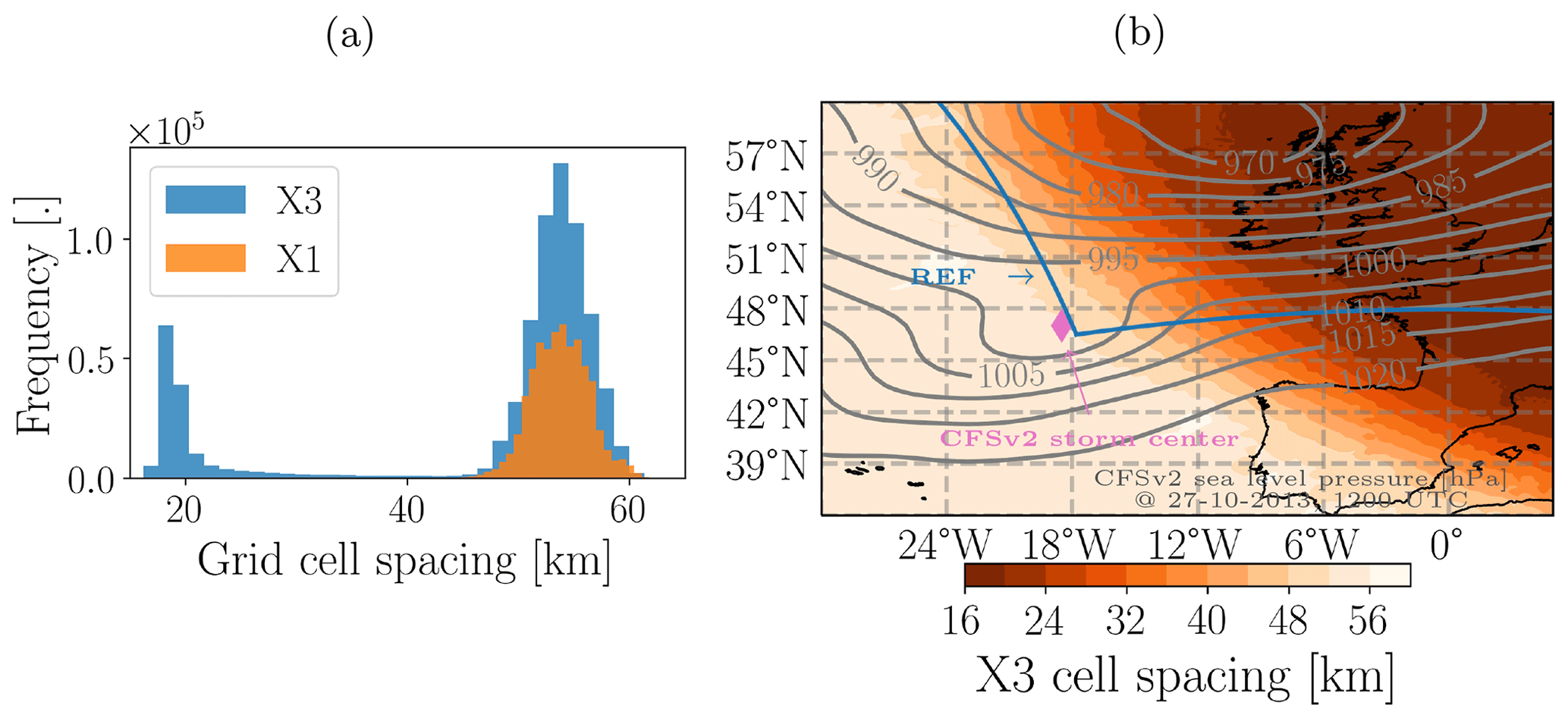
Figure 4 (a) Histogram of grid cell distances in the quasi-uniform X1 and variable-resolution X3 MPAS mesh configuration. (b) Spatial distribution of grid cell spacing in the X3 mesh configuration together with the sea level pressure contours and storm center location obtained from CFSv2 at 27 October 2013, 12:00 UTC as well as the “REF” domain from WRF. The presence of grid spacing below 18 km in X3 is a consequence inherent to MPAS' SCVT mesh discretization which requires deviations in grid cell sizes of individual cells also below the target to maintain SCVT properties (see e.g. Du et al., 2003; Ringler et al., 2008 for details).

(Niu et al., 2011; Yang et al., 2011)

Table 3 Overview of MPAS scenarios and their configuration. Used abbreviations: KF: Kain-Fritsch (Kain, 2004), GF: Scale–aware Grell–Freitas (Grell and Freitas, 2014), NT: New Tiedtke (Zhang et al., 2011; Zhang and Wang, 2017), TMS: Thompson non-aerosol aware (Thompson et al., 2008), WSM6: WRF Single–Moment 6-Class (Hong and Lim, 2006), MYNN: Mellor–Yamada–Nakanishi–Niino (Nakanishi and Niino, 2009), YSU: Yonsei University Scheme (Hong et al., 2006), MM5: Revised MM5 similarity scheme (Jiménez et al., 2012), RRTMG: Rapid Radiative Transfer Model for General Circulation Models (Iacono et al., 2008).

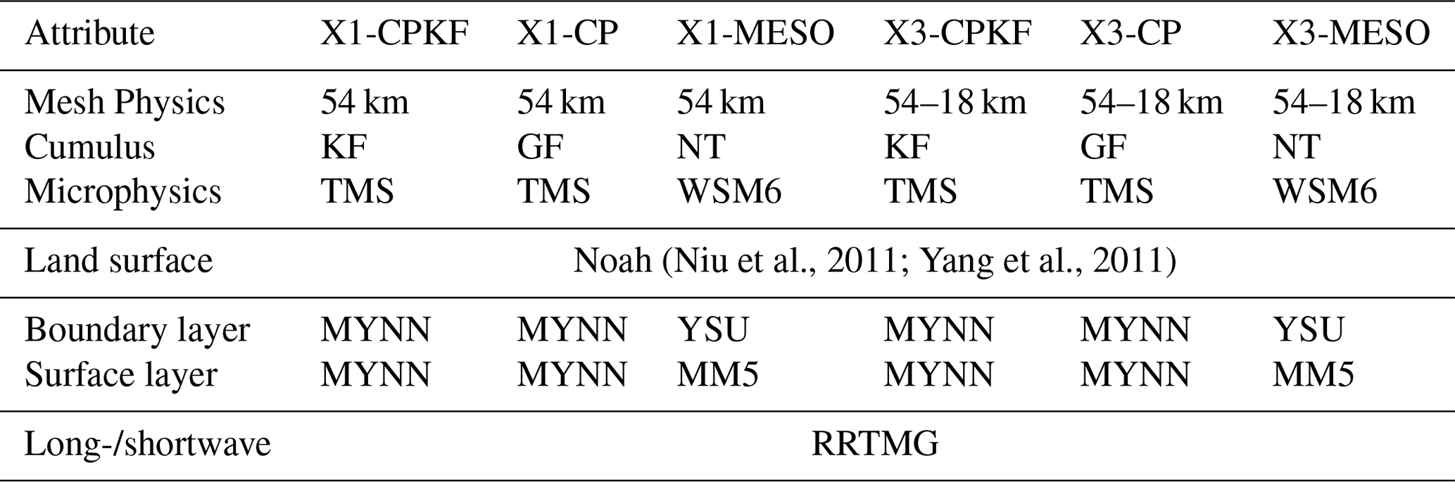
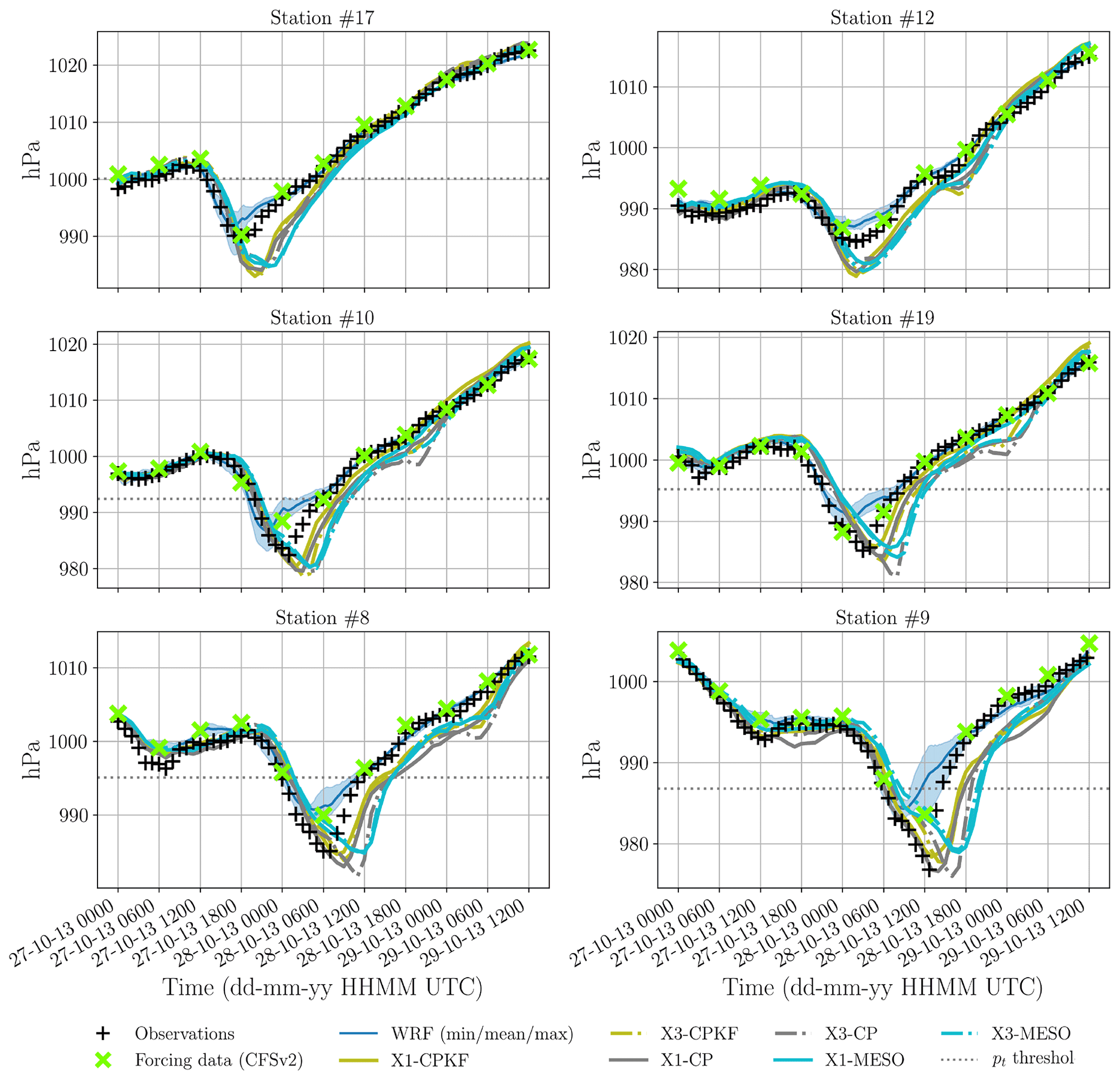
Figure 5 Time series of sea level pressure at the six buoy locations obtained from observations, CFSv2 forecast data, the extended WRF simulations described in Sect. 2.3 and the six MPAS configurations. To highlight the difference between the individual MPAS configurations and WRF, the results from the seven WRF configurations are aggregated and represented as average values and an interval enclosing minimum and maximum values for each data point. The naming of the MPAS configurations follows the naming convention introduced in Table 3.

3 Results

3.1 MPAS in Comparison with WRF, CFSv2 and Observations

Figure 5 depicts the time series of the sea level pressure during the impact period of Christian at the locations of the buoy. To highlight the differences in performance between MPAS and WRF in the time series, the results from the seven WRF configurations are aggregated and represented as average values surrounded by an interval enclosing the minimum and maximum of the seven simulations for each data point. While the different modeling approaches show generally good agreement with the observations, major differences are visible at the time of impact of storm Christian and afterwards. It can be seen that WRF is generally not able to deepen the low pressure system enough compared to the measurements. This can be seen more clearly in Fig. 6a, which shows the difference in storm intensity as introduced in Sect. 2.1 between the models and the buoy observations. WRF is generally underestimating the local minimum sea level pressure with the exception of the very frequently updated versions CFSv2-3h and CFSv2-1h at station #17. One reason can be attributed to the performance of the CFSv2 product that has been used as driving boundary conditions. While the forcing data agrees well in the timing of the local minimum sea level pressure, it has difficulties in adequately representing the sea level pressure drop associated with storm Christian at later stages of the storm. This is especially visible at stations #10, #8 and #9 (Fig. 5a). While the spread between the individual WRF configurations is large, the different approaches of how the boundary conditions are introduced (cf. Table 2) can balance this only to a certain extend. Far away form the storm impact (temporally and spatially spoken), the good agreement between CFSv2 and the observations keeps the limited area model WRF in line with the measurements and the spread between the WRF model configurations is strongly reduced (e.g. before and after approximately 6 h after the station sees its LMSLP, Fig. 5). As visible in Fig. 5, the differences between the individual WRF simulations become mostly relevant only in the vicinity of the storm center which has been analyzed in detail in Imberger et al. (2020).

Figure 6 Difference in (a) storm intensity, (b) t_LMSLP and (c) storm duration between the simulations and the buoy observations. The naming of the WRF and MPAS configurations follows the naming convention introduced in Tables 2 and 3, respectively.

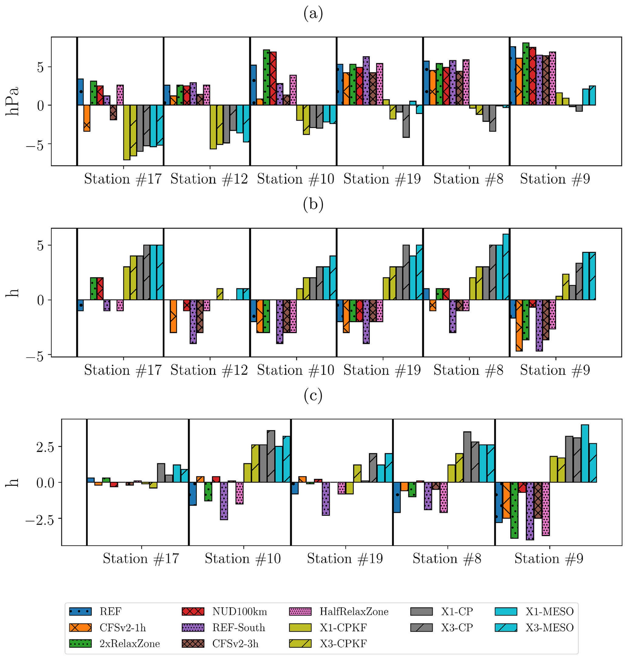
The global MPAS simulations on the other hand are not influenced by external data with the exception of the model initialization, which originates from the same CFSv2 product as the WRF simulations (see Sect. 2). A closer look around the different LMSLPs shows that MPAS has better agreement in the representation of the pressure drop associated with storm Christian at stations #10, #19, #8 and #9 (Fig. 5). This results in lower deviations in the modeled storm intensity as defined in Sect. 2.1 (cf. Fig. 6a) at those stations compared to WRF. However, an underestimation of the sea level pressure for times after t_LMSLP is observed in all MPAS configurations with similar magnitude (e.g. time series after 28 October 2013, 06:00 UTC at station #8, cf. Fig. 5). This period is also characterized by the highest spread between the different MPAS physics and mesh configurations and the period where deviations from the buoy observations are the largest. Looking at the differences in t_LMSLP as defined in Sect. 2.1 (Fig. 6b) reveals different patterns in WRF and MPAS. While the majority of WRF configurations estimate t_LMSLP too early compared to the measurements (i.e. negative difference in t_LMSLP up to approximately 5 h), MPAS overall determines t_LMSLP too late with some exception at station #12. This is partly attributed to a general westward-shift of storm Christian within MPAS compared to the CFSv2 data that has been observed independently from the physics and mesh settings. Due to the observed underestimation of the sea level pressure after t_LMSLP, differences in storm duration as defined in Sect. 2.1 (cf. Fig. 6c) are also higher in most cases compared to the observation.

3.2 Impact of MPAS Mesh Refinement and Model Physics

Comparing the different MPAS variable-resolution configurations with their quasi-uniform counterpart, a small degradation of the model performance with respect to t_LMSLP is observed in the variable-resolution simulations. Times of local minimum sea level pressure are generally estimated equally late or even later in the variable-resolution simulations independently from the chosen physics configuration (Fig. 6b). This can be attributed to a combination of an additional west-wards shift and the development of a tail of extended lower pressure resulting in a stretch of the storm structure in southwestward direction (see example for 28 October 2013, 06:00 UTC in Fig. 7). These effects are present in the variable-resolution configurations with different severity depending on the physics configuration used. The additional west-ward shift is strongly developed in the CPKF and CP physics configurations (Fig. 7a, b), resulting in a delayed arrival time at five out of the six stations along the travel path (Fig. 6b). Differences in the storm location are less pronounced in the MESO configuration (Fig. 7c), but due to the southwestern tail of extended low pressure (around 5.4^∘ W), stations that are located in the southwestern wake of the storm structure (e.g. station #10, #19 and #9 in the south of England) will experience their LMSLP pressure later. It must be noted that the storm center in X1-MESO is already located further southwest than the corresponding X1-CPKF and X1-CP configurations suggest (cf. Fig. 7) resulting in the overall, on-average, highest difference in t_LMSLP (Fig. 6b) compared to the other two physics settings. Worth mentioning is that X3-CP also shows an extended low pressure region southwest of the storm center in addition to the west-wards shift that is additionally contributing to a later t_LMSLP in this configuration.

Figure 7 Contours of sea level pressure (in hPa) of variable-resolution (X3) and quasi-uniform (X1) MPAS configurations for a given set of model physics at 28 October 2013, 06:00 UTC: (a) the -CPKF, (b) -CP and (c) -MESO physics configuration. Contours are drawn from 973 to 990 hPa with 1 hPa intervals. Naming of the MPAS configurations follows Table 3.

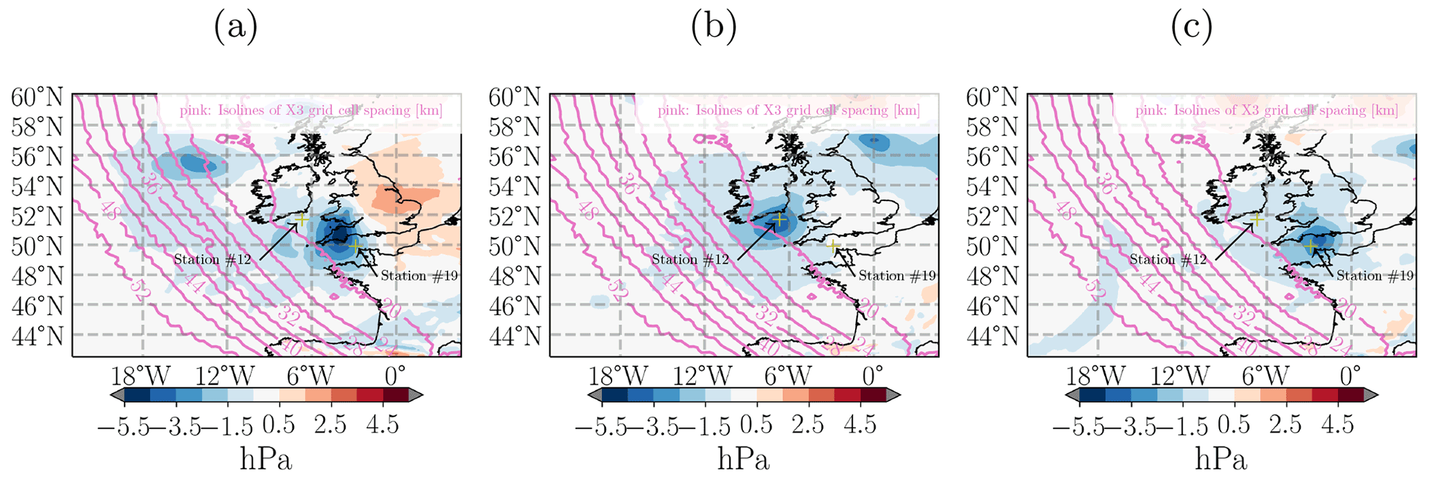
Figure 8 Difference of sea level pressure between X3-CPKF and X1-CPKF at (a) 28 October 2013, 06:00 UTC, (b) 28 October 2013, 18:00 UTC and (c) 29 October 2013, 00:00 UTC exemplifying the propagation of the small low pressure system from the North Atlantic towards south-east. Station #12 and #19 as well as the mesh transition zone of the X3 mesh configuration are depicted for reference.

While the mesh refinement has not helped to improve the results with respect to the three defined storm metrics of Christian, only the variable-resolution configurations captured the plateau of more or less constant sea level pressure at station #12 (Fig. 5). This is also visible to a smaller degree at station #10 and station #8. An analysis of the time series of the spatial sea level pressure of all variable-resolution configurations suggests that this effect originates from a small low-pressure system that develops in the North Atlantic within the transition zone region of the mesh (Fig. 8a) and that moves south-eastward (Fig. 8b, c). While the timing and magnitude of the phenomena are slightly off compared to the observations, the refined configurations are able to develop the pressure plateau seen at station #12 (Fig. 5b). Information from the observations about the actual travel path are somewhat inconclusive due to the presence of the pressure plateau at stations #10 and #8, while being absent at #19 (which is located in between station #10 and #8, cf. Fig. 2). This makes it challenging to clearly identify the actual travel path. Interestingly, X1-CP also shows indications of a pressure plateau at station #19 (cf. Fig. 2d) similar to X3-CPKF, X3-MESO and X3-CP, but due to its absence at both station #8 and #10 in the model results it is likely not attributed to the same underlying moving system. It must be noted that the observations at station #19 do not suggest the presence of a pressure plateau and that the quasi-uniform X1-MESO and X1-KF configurations actually agree better at this station with the measurements around 29 October 2013, 00:00 UTC.

4 Discussion

The results have shown that MPAS is generally able to represent storm intensity for the presented case, but challenges have been identified in the estimation of t_LMSLP and storm duration. The poorer performance with respect to t_LMSLP and storm duration was caused by a superposition of a general west-ward shift of the MPAS forecast compared to the real atmospheric state (affecting all MPAS forecasts) and an additional south-westward shift and/or an artificially extended low pressure zone in the south-west of the storm center in the variable-resolution configurations (cf. Fig. 7). While the negative effects associated with lateral boundary conditions (spatial and temporal interpolation, see discussion in Imberger et al., 2020) that were observed in the WRF simulations are avoided with MPAS, the freedom associated with the lack of lateral boundary conditions allowed the west-ward shift of the storm structure at an early stage. That shift was not corrected due to the models independence after model initialization. This highlights that other means of constraining the global model integration, like data assimilation techniques, might be necessary to replace the beneficial effect of lateral boundary conditions of constraining the model integration.

Despite MPAS' capabilities to define smooth transition zones for mesh refinement to avoid storm structure distortion caused by e.g. the corner issue discussed in Imberger et al. (2020), the additional west-ward shift and/or extended low pressure zone (cf. Fig. 7) in the variable-resolution configurations has shown that smooth transition zones alone might not always be sufficient to completely remove storm displacements or distortions in large-scale fields like the sea level pressure. This underlines that dealing with complex atmospheric structures like mid-latitude storms in a variable-resolution environment remains a very challenging task that needs further understanding about the interaction between grid spacing, model dynamics and physics to adequately represent the storm structure. While the mesh refinement has not improved the results with respect to the key storm metrics, it must be noted that the sea level pressure as a large-scale storm feature (Hoskins and Hodges, 2002) can not provide a full picture of potential benefits of the mesh refinement. It is expected that these benefits would be more pronounced in small-scale atmospheric variables like relative vorticity or wind speed. However, lack of suitable observational data adequate for the given grid spacing in this period limited further validation for these variables.

5 Conclusions

As case study of a mid-latitude storm has been simulated with the global Model for Prediction Across Scales with both variable-resolution and quasi-uniform mesh configurations as well as different physics settings. MPAS' performance has been evaluated against buoy observations with respect to key storm metrics such as storm intensity, t_LMSLP and storm duration. MPAS is able to adequate represent storm intensity based on local minimum sea level pressure while model drift and impacts of mesh refinement caused displacement of the storm structure compared to observations and external forecast products. The study highlights the need for data assimilation techniques to counteract model drifts due to missing regular model updates.