 | 17 Dec 2020
Benchmark data for verifying background model implementations in orbit and gravity field determination software
Martin Lasser
Ulrich Meyer
Adrian Jäggi
Torsten Mayer-Gürr
Andreas Kvas
Karl Hans Neumayer
Christoph Dahle
Frank Flechtner
Jean-Michel Lemoine
Igor Koch
Matthias Weigelt
Jakob Flury
In the framework of the COmbination Service for Time-variable Gravity fields (COST-G) gravity field solutions from different analysis centres are combined to provide a consolidated solution of improved quality and robustness to the user. As in many other satellite-related sciences, the correct application of background models plays a crucial role in gravity field determination. Therefore, we publish a set of data of various commonly used forces in orbit and gravity field modelling (Earth's gravity field, tides etc.) evaluated along a one day orbit arc of GRACE, together with auxiliary data to enable easy comparisons. The benchmark data is compiled with the GROOPS software by the Institute of Geodesy (IfG) at Graz University of Technology. It is intended to be used as a reference data set and provides the opportunity to test the implementation of these models at various institutions involved in orbit and gravity field determination from satellite tracking data. In view of the COST-G GRACE and GRACE Follow-On gravity field combinations, we document the outcome of the comparison of the background force models for the Bernese GNSS software from AIUB (Astronomical Institute, University of Bern), the EPOS software of the German Research Centre for Geosciences (GFZ), the GINS software, developed and maintained by the Groupe de Recherche de Géodésie Spatiale (GRGS), the GRACE-SIGMA software of the Leibniz University of Hannover (LUH) and the GRASP software also developed at LUH. We consider differences in the force modelling for GRACE (-FO) which are one order of magnitude smaller than the accelerometer noise of about 10−10 m s−2 to be negligible and formulate this as a benchmark for new analysis centres, which are interested to contribute to the COST-G initiative.
- Article
(265 KB) - Full-text XML
- BibTeX
- EndNote


The correct application of background models plays a crucial role in many satellite-related sciences, such as orbit and gravity field determination. Nowadays not only one software is used to perform such tasks but various institutions around the world have set up their own processing schemes based on their in-house developed software packages. In order to minimise systematic differences caused by a diverse handling of well established models, for example, background force models, the effort of comparing software implementations is picked up regularly. Software comparisons are always a useful tool for detecting inconsistencies or even bugs in software implementations.
In the framework of the COST-G (Jäggi et al., 2020) gravity field solutions from different analysis centres (ACs) are combined to offer a consolidated solution of improved quality, robustness and reliability to the user. As the example of several services, like the International GNSS Service (Johnston et al., 2017) and the International Laser Ranging Service (Pearlman et al., 2002), showed, combining solutions from various institutions, which are computed by different and independent software packages, leads to improved results. The COST-G initiative was formally established in 2019 and operationally provides state-of-the-art monthly global gravity models from the Gravity Recovery And Climate Experiment (GRACE, Tapley et al., 2004), GRACE Follow-On (Landerer et al., 2020) and Swarm (Friis-Christensen et al., 2006). COST-G is a product centre of the International Gravity Field Service (IGFS) under the umbrella of the International Association of Geodesy (IAG).
Modelling background forces is vital to gravity field determination, especially when the time variable part is considered. Therefore, we publish a set of data of various commonly used forces in orbit and gravity field modelling evaluated along a one day orbit arc of GRACE, together with auxiliary data to enable easy comparisons. This data set is intended to be used as a reference data set and provides the opportunity to test the implementation of these models in various software packages. The COST-G consortium consists at the time of writing of ACs and further candidate ACs. Thus, we took the opportunity to test several software packages available within the COST-G consortium, which are the Bernese GNSS software (Dach et al., 2015) from AIUB (Astronomical Institute, University of Bern), EPOS (Zhu et al., 2004) of the German Research Centre for Geosciences (GFZ), the GINS software, developed and maintained by the Groupe de Recherche de Géodésie Spatiale (GRGS), the GRACE-SIGMA (Koch et al., 2020) software of the Leibniz University of Hannover (LUH) and the GRASP software (Weigelt et al., 2013) from LUH. Furthermore, we use this reference data to set a benchmark for new analysis centres, which are interested to contribute to the COST-G initiative.
The paper is organised in five sections, where Sect. 2 introduces the data set used and published in this study. Section 3 summarises the evaluation of each force model, intended to be easily comprehensible for programming. We discuss the result of a force comparison for one software package in more detail in Sect. 4 and give the summarised outcome of the comparisons for all COST-G ACs and candidate ACs. Finally, Sect. 5 concludes the results of this study and highlights the importance beyond the COST-G group.
The benchmark data set was compiled at the Institute of Geodesy (IfG) at Graz University of Technology. It consists of several accelerations a spacecraft experiences, evaluated along a given orbit, which are commonly used in orbit and gravity field determination. The models that describe the accelerations are evaluated along a one day GRACE orbit arc (integrated for 3 July 2008 using Encke's method, see Ellmer and Mayer-Gürr (2017) for more information on the integration) using the GROOPS software. The orbit has a 30 s sampling and is given in cartesian coordinates expressed in both Terrestrial Reference Frame (TRF), where ITRF2014 (Altamimi et al., 2016) is used, and the Celestial Reference Frame (CRF), where ICRF2 (Fey et al., 2009) is taken. The evaluations yield three dimensional accelerations for each sampling point at the location of the spacecraft. These accelerations are the main product of the benchmark data set. The underlying models are listed in Table 1.
Table 1Accelerations modelled in the benchmark data set. The magnitude is a rough estimation for the given GRACE orbit, the list is ordered according to the magnitude of the forces.
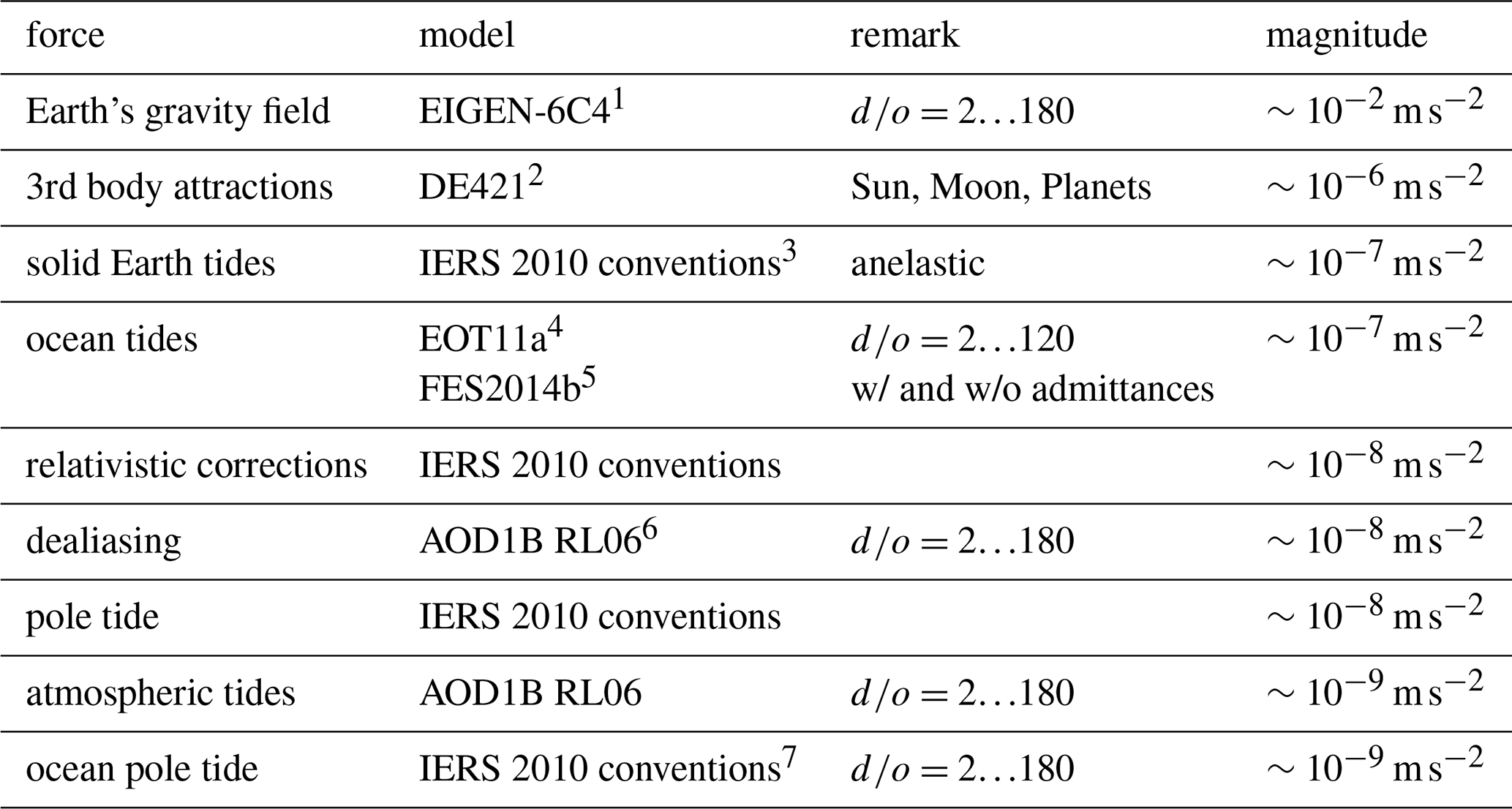
1 Förste et al. (2014). 2 Folkner et al. (2009). 3 Petit and Luzum (2010). 4 Savcenko and Bosch (2011). 5 Carrere et al. (2016). 6 Dobslaw et al. (2017). 7 Desai (2002).
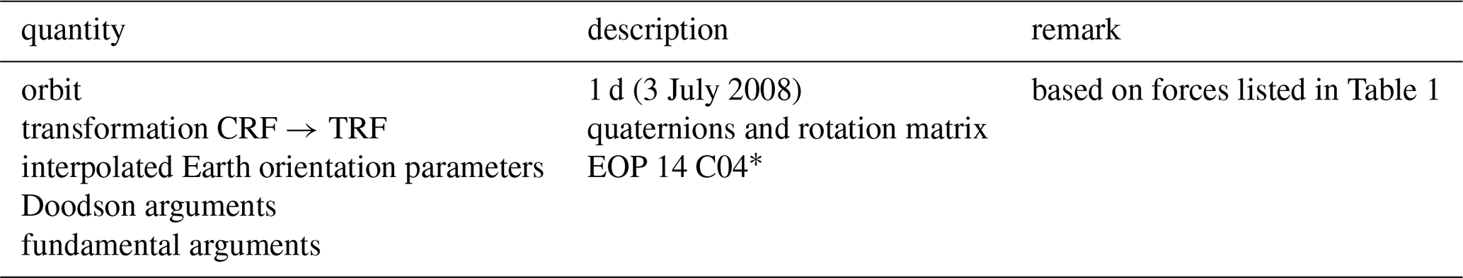
All resulting accelerations are expressed in the CRF, the gravity field is additionally given in TRF. For each acceleration one file is provided. Accelerations consisting of several components, such as ocean tides, are provided in separate files for the largest constituents. Each file provides time stamps in GPS time (expressed in Modified Julian Date [MJD]) and the respective x, y, z-accelerations. As the definition of frames may vary between different software packages (J2000, true system of epoch), the orbit is given in the terrestrial and the celestial reference frame, and additionally, the rotation between the two underlying frames is provided as quaternions and rotation matrices. In an attempt to also make the handling of the terrestrial and celestial reference frame comprehensible, as well as to enable an easier understanding of ocean and atmosphere tide models, several additional physical quantities are appended to the data set.
The additional data is listed in Table 2.
The complete data set can be found at the ftp server of IfG1 including a description of the data and how the models are employed (see file 00README_simulation.txt).
To illustrate the nature of the accelerations Fig. 1 shows the norm of each acceleration considered in the benchmark data in CRF. The mean orbital altitude is 466 km.

2.1 Application of the benchmark data set
The main goal of the data is to provide a reference for basic software comparisons. It enables a comparison of the background force model implementations by evaluating the models at the given orbital positions in different software packages, and may serve as a reference for the handling of celestial and terrestrial reference frames. The most straight forward approach of comparison is to evaluate the force models with a given space geodesy software package and to print the resulting accelerations for each model. By subtracting the obtained accelerations from the benchmark data, differences may be revealed
d denotes the difference between the reference and the software under evaluation, r the reference accelerations and s the accelerations resulting from the software's evaluation. Large differences to the reference accelerations may indicate potential implementation problems. It is very unlikely to obtain zero differences. Unless large systematic differences emerge, oscillating patterns around zero will usually be observed due to the orbital revolution, most commonly twice-per-revolution due to the Earth's oblateness at the poles and the almost polar reference orbit.
In the following we also use the maximum absolute deviation from the reference (dmax) to summarise the comparisons of several software packages
In this section we give a few notes on each force in the benchmark data set. All formulae correspond with the IERS 2010 conventions (Petit and Luzum, 2010), however, they are provided in the way they are coded in the Bernese GNSS software. All constants can be found in the IERS 2010 conventions and the corresponding model descriptions. When referring to the equations from the IERS 2010 conventions we use the notation Eq.IERS (n.n) to provide good reading flow.
3.1 Earth's Gravity field
The gravity field model used for the benchmark data set is EIGEN-6C4 (Förste et al., 2014), which contains a set of dimensionless, fully-normalised spherical harmonic coefficients representing the static part of the Earth's gravity field. In the benchmark accelerations it is evaluated from degree and order 2 to 180. In contrast to all other forces, the data set contains the accelerations expressed in both CRF and TRF. The Earth's potential and the coefficients are related by
where cnm and snm denote the normalised spherical harmonic coefficients of degree n and order m and Pnm are the normalised associated Legendre functions. The point of calculating the potential is defined by the spherical coordinates with the radius r, the co-latitude ϑ and the geographical longitude λ. aE defines the reference radius of the Earth, GME the gravitational constant multiplied with the mass of the Earth. Both are associated with the gravity field model and can be found in the header of EIGEN-6C4 data file. Equation 3 corresponds to Eq.IERS (6.1).
The accelerations and the potential are related by
with ∇ being the gradient operator. The accelerations in cartesian coordinates can be obtained by a transformation of Earth-fixed ()-frame to ()-frame. We refer to Heiskanen and Moritz (1967) for a detailed derivation of the expression of the Earth's gravity field in spherical harmonics.
3.2 3rd body attractions
The influence of other celestial bodies (denoted by the subscript cb) than the Earth is computed with positions derived from the JPL DE421 (Folkner et al., 2009) ephemeris. All bodies are treated as point masses, thus,
expresses the accelerations caused by a celestial body. rsat and rcb denote the geocentric position vector of the satellite and the celestial body. The constants of GMcb are given in the readme-file. Planets up to Saturn are taken into account, however, as tests showed, additionally introducing Neptune, Uranus and Pluto leads to negligible small differences. The positions of Sun and Moon, computed from the DE421 ephemeris, are also used for the Solid Earth tides and the relativistic corrections.
3.3 Solid Earth tides
Solid Earth tides are computed according to IERS 2010 conventions using the anelastic model. Besides fundamental quantities of the Earth, the solid Earth tides depend on the position of the Sun, the Moon and the load Love numbers. They affect the spherical harmonic spectrum up to degree four.
According to the IERS 2010 conventions the computation is divided into two steps. Step 1 computes the coefficients due to the tide generating potential for degree 2 and 3, as well as the effect of degree 2 on degree 4 coefficients. Step 1 is frequency independent, whereas step 2 states frequency dependent corrections for degree two.
Step 1 – corresponds with Eqs.IERS (6.6) and (6.7):
, , denote the Love numbers (TableIERS 6.3), rS and rM is the norm of the geocentric vector (rS, rM) to Sun and Moon, the Legendre functions Pnm depend on the cosine of the co-latitude ϑS,M of Sun and Moon in the TRF. λS,M is the geographical longitude of Sun and Moon in the Earth-fixed frame.
Step 2: Corrections on c20 – corresponds to Eq.IERS (6.8a) and uses TableIERS 6.5b:
Corrections on c21, c22, s21, s22 – corresponds to Eq.IERS (6.8b) and uses TableIERS 6.5a and TableIERS 6.5c:
The amplitudes for the frequency dependent corrections for and are listed in TablesIERS 6.5a, 6.5b and 6.5c.
The Doodson angle argument reads as
with θf being computed from the fundamental Doodson arguments β and the respective tidal frequency nf. Both vectors have six elements. The computation of the fundamental Doodson arguments follows from the fundamental arguments of lunisolar nutation (Delaunay variables, cf. Doodson and Lamb, 1921) (Eq.IERS (5.43)).
t denotes the time interval between the current epoch and J2000.0 in Julian centuries, thus,
Finally, the Doodson arguments read as
where θg denotes Greenwich Mean Sidereal Time (GMST) in angle units.
In the tidal frequency vector nf each digit makes up one element of the multipliers ni, the representation is hexadecimal to allow for frequencies greater than 999.999. An example for the long periodic om1-tide with a frequency of 55.565 would be . The first element of the vector tells the periodicity of the tide.
The final coefficients and are obtained by adding together step 1 and step 2
In order to provide all information needed for the evaluation, the Doodson arguments and fundamental arguments of nutation, computed for every position of the reference orbit, are also part of the data set. They are also needed for the computation of ocean and atmospheric tides. The accelerations caused by the solid Earth tides are eventually computed using Eqs. 3 and 4.
3.4 Ocean tides
Two different models are provided for the ocean tides: EOT11a (Savcenko and Bosch, 2011) and FES2014b (Carrere et al., 2016). Both are based on IfG's conversion of the corresponding grids to spherical harmonic coefficients. EOT11a is evaluated from degree 2 to 120, FES2014b from degree 2 to 180. EOT11a consists of 18 tidal frequencies, FES2014b of 34. Furthermore, the data set provides linear admittances, a short description and a MATLAB routine of their application. The spherical harmonics coefficients can be computed from the given prograde (, ) and retrograde (, ) coefficients in a sum over all tidal frequencies f using
In this representation the Doodson-Warburg correction (see TableIERS 6.6) is already applied.
To complete the tidal spectrum, admittances between the major tides can be computed using linear interpolation
The subscripts 1 and 2 denote the main waves, f the interpolated wave. H is the astronomic amplitude of the wave. The ocean tides are given in ICGEM-format (Barthelmes and Förste, 2011, “.gfc”) and IERS-format. The latter provides a smaller number of significant digits for the coefficients, hence, we expect differences at the level of 10−11 m s−2 when using the two different file formats. The tidal frequencies and the phase shift applied (Doodson-Warburg correction) are stated in the readme-file. For the evaluation using the IERS-format (potential and water height) we refer to Petit and Luzum (2010, chap. 6.3.1). Accelerations resulting from ocean tides are eventually obtained by Eqs. (3) and (4).
3.5 Relativistic corrections
Relativistic corrections are computed according to the IERS 2010 conventions for General Relativity using Eq.IERS (10.12) and contain the Schwarzschild (Eq. 19), Lense-Thirring (Eq. 20) and de Sitter term (Eq. 21).
rsat and vsat are the geocentric position and the velocity of the satellite. c denotes the speed of light, J is the Earth's angular momentum per unit mass and can be set to m2 s−1 (Petit and Luzum, 2010). The vectors rS and vS describe the geocentric position and velocity of the Sun in CRF. The relativistic accelerations in the benchmark data are the sum of the three components
3.6 Dealiasing
AOD1B RL06 (Dobslaw et al., 2017) is used as dealiasing product. The “glo” dataset, which is the sum of the atmospheric and oceanic contribution, is evaluated in the benchmark data. The degree one coefficients are not taken into account, it is evaluated from degree 2 to 180. The spherical harmonic synthesis of the dealiasing model follows Eqs. 3 and 4, additionally, as the data set is given in three hour sets, a linear interpolation between the neighbouring sets at time t1 and t2 is performed on the level of spherical harmonic coefficients to obtain the spherical harmonic coefficients at time ti () (Eq. 23).
3.7 Pole tide
“The pole tide of the solid Earth is generated by the centrifugal effect of polar motion” (Petit and Luzum, 2010, chap. 6.4). Only the coefficients c21 and s21 are concerned and the contribution is computed from the polar motion parameters and the mean pole definition via
xP, yP, and form the wobble parameters (Eq.IERS (7.24)) via
The pole tide and ocean pole tide computed in the benchmark data make use of the most recent secular pole (IERS, 2018)
in units of arc seconds with t denoting the time interval between the current epoch and J2000.0 in Julian years, thus,
The relation between the spherical harmonic coefficients and the accelerations is again given by Eqs. 3 and 4.
3.8 Atmospheric tides
Atmospheric tides are modelled using AOD1B RL06 product and contain all twelve tidal constituents from degree 2 to 180. Additionally, the accelerations caused by S1 tide only are given separately. The evaluation of the atmospheric tides follows
where the coefficients , , , are given by the model for each tidal frequency f. The angle argument θf follows from Eq. (12), the Doodson-Warburg phase correction χf depends on the tidal frequency. To obtain accelerations, the spherical harmonic coefficients can be evaluated by using Eqs. (3) and (4).
The model is given in ICGEM-format as well. Using this format, the application follows the method described for the ocean tides (see Eq. 17). For the evaluation using the IERS-format (potential) we refer to Petit and Luzum (2010, chap. 6.3.1).
3.9 Ocean pole tide
Similar to the solid Earth pole tide, the ocean pole tide is a result of the centrifugal effect of polar motion on the oceans. The implementation for the benchmark data set follows the IERS 2010 conventions employing the Desai model (Desai, 2002), which is given in spherical harmonic coefficients, representing a self-consistent equilibrium model. The benchmark accelerations make use of the degrees and orders 2 to 180. Load Love numbers are given externally as the conventions only state a few of the low degree Love numbers. The formulae follow Eqs.IERS (6.23a) and (6.23b).
where , , , are the coefficients from the model, m1 and m2 are the wobble parameters (Eq. 25), , and the factor Rn is given by
with ωE being the nominal mean Earth's rotation velocity, G the gravitational constant, ρ the density of sea water, geq the gravity at the equator and the load Love numbers. To obtain accelerations, the spherical harmonic coefficients are evaluated using Eqs. (3) and (4).
The benchmark data set was created, used and examined within the COST-G initiative, where AIUB, GFZ, GRGS and IfG are currently acting as COST-G ACs. LUH is a candidate AC. To augment the combination effort and in particular to rule out large systematic differences in the implementation of background force models, all contributing groups performed a comparison with the benchmark data using their own software packages. This includes the Bernese GNSS software (AIUB), EPOS (GFZ), GINS (GRGS), GROOPS (IfG), GRACE-SIGMA (LUH) and GRASP (LUH). The intention of this comparison is to test the implementation and handling of the background models in each software package. Every software tries to reproduce the reference accelerations as closely as possible by employing the provided rotation between TRF and CRF. The GROOPS software serves as a reference as it was used to compute the benchmark data set.
4.1 Software packages
The software packages follow different approaches of modelling gravity fields from satellite data. Even though data is treated differently, we expect a high level of agreement with the benchmark data for background model handling. The following sub-sections give a brief introduction to each package.
4.1.1 Bernese GNSS software
The Bernese GNSS software is a scientific software package, used by more than 700 institutions around the world. It features space geodetic applications, mainly high-precision, multi-GNSS data processing for ground networks (e.g., Prange et al., 2017) as well as precise satellite orbit determination and thereof deriving gravity field solutions (e.g., Meyer et al., 2016). The software is developed, maintained and distributed at AIUB. In its core it employs the Celestial Mechanics Approach of orbit determination, be it for high or low flying Earth orbiting satellites or planetary geodetic applications (Arnold et al., 2015). The software is written in Fortran.
4.1.2 EPOS
The Earth Parameter and Orbit System (EPOS2) is a software package designed and used for operational Precise Orbit Determination (POD). It consists of tools for data orbit analysis, orbit integration, orbit improvement, orbit predictions, normal equation handling and simulation of observations, as well as for gravity field computation. It served and serves numerous satellite missions, such as Mir, Space Shuttle, LAGEOS, CHAMP, GRACE, GOCE, GRACE-FO, Swarm, TerraSAR-X, TanDEM-X, Envisat or Jason, being able to deal with SLR, GPS, DORIS, radar altimeter or GRACE K-Band-Ranging data. EPOS is based on the dynamic approach of orbit modelling and EPOS is one of the software of the current COST-G ACs that is written in Fortran. EPOS is developed, maintained and used at GFZ, and has also been installed at a few other institutions around Europe. Recent applications are the computation of monthly GRACE and GRACE-FO gravity field solutions (Dahle et al., 2019) or investigations on local ties for the datum realisation of global terrestrial reference frames (Glaser et al., 2019).
4.1.3 GINS
The GINS (Géodésie par Intégrations Numériques Simultanées) software is developed and maintained by the GRGS of the French space agency. It is a multi-technique space geodetic software, capable of processing data from GNSS, SLR, VLBI, DORIS and inter-satellite ranging. It is used for operational processing of all space geodetic observation techniques.
4.1.4 GRACE-SIGMA
The GRACE-SIGMA (GRACE-Satellite orbit Integration and Gravity field analysis in MAtlab) software is a recent development specifically designed for the processing of GRACE and GRACE-FO data. The software is developed at Institut für Erdmessung (IfE) of LUH. It is written entirely in MATLAB and uses strongly vectorised modules for modelling of disturbing forces, orbit propagation and orbit improvement. The integration of satellite ephemerides and state and sensitivity matrices is performed using an efficient in-house developed numerical integration approach (Naeimi, 2018). The gravity field estimation is based on a generalized dynamic orbit determination using variational equations. The software is applied for the computation of monthly GRACE and GRACE-FO gravity field solutions (Koch et al., 2020).
4.1.5 GRASP
The GRAvity Satellite Processing engine (GRASP) software is dedicated to gravity field recovery from kinematic positions of satellites (Weigelt et al., 2013). It uses the acceleration approach of orbit modelling, thus, the kinematic positions are numerically differentiated twice in order to make them express a quantity directly related to the force field that is acting on the satellite. GRASP is developed at LUH and written in MATLAB.
4.1.6 GROOPS
The Gravity Recovery Object Oriented Programming System (GROOPS) used at IfG is a software suite for geodetic applications. Its feature set includes the determination of GNSS orbits, clocks and ground station networks (Strasser et al., 2019), static and time-variable gravity field solutions from satellite data, and regional gravity field modeling with terrestrial data. GROOPS is written in C++ and makes heavy use of low level Basic Linear Algebra Subprograms (BLAS) and LAPACK (Linear Algebra PACKage) subroutines. It uses the Message Passing Interface (MPI) communication protocol for parallelization and is therefore capable to run on large distributed systems. GROOPS software serves as a reference within these software comparisons as the benchmark data set was compiled using the capabilities of GROOPS. Recent applications are the computation of the ITSG‐Grace2018 time series (Kvas et al., 2019) and operational processing of GRACE-FO data.
4.2 Example results using the Bernese GNSS Software
To show the results of the software comparison for all provided force models, we evaluate all force models with the Bernese GNSS software and compute the norm of the difference vector between the benchmark accelerations and the accelerations from Bernese. We expect the magnitude of the differences to be small as the handling of the background forces is supposed to be generally compatible. Figure 2 shows that the largest differences result for the solid Earth tides, the smallest for the relativistic effects. Generally, the magnitude of differences is close to the numerical precision of 64 bit arithmetic of about 16 decimal places (IEEE-754, 1985).
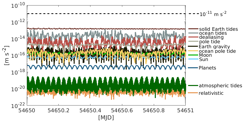
Figure 2Norm of the difference between the benchmark data and the evaluation with the Bernese GNSS software.
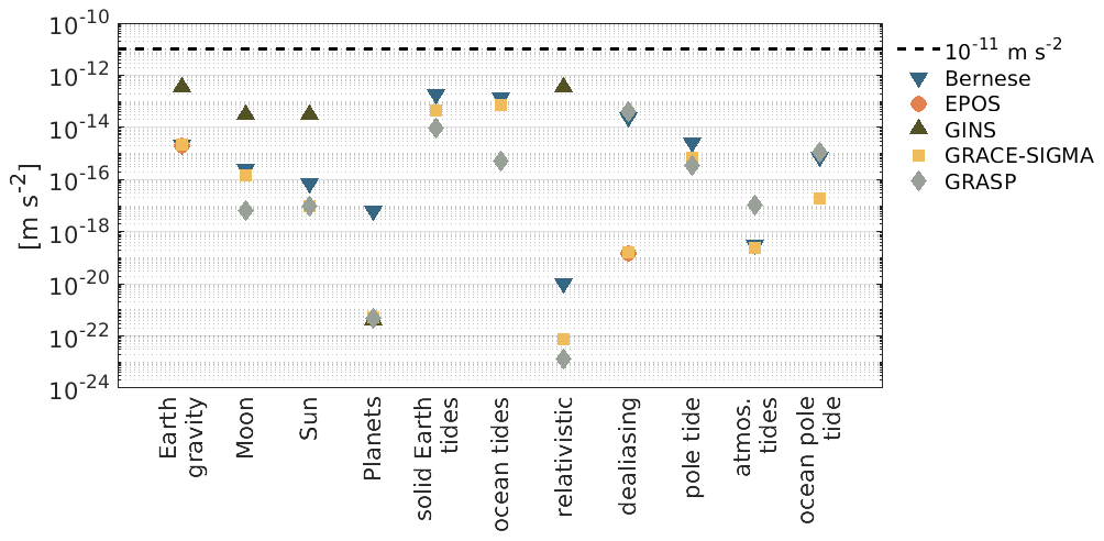
Figure 3Maximum absolute deviation of the difference between the reference and the evaluation by the respective software of the COST-G ACs for each force considered in the benchmark data set.
4.3 Results from COST-G
Each of the above mentioned institutions performed the software comparison with the benchmark data. EPOS and GINS currently contribute only with a subset of forces, whereas all others accomplished the comparison for all accelerations provided in the reference data set. The limit for the difference in evaluating the models along the reference orbit was set to 10−11 m s−2, thus, at least one order of magnitude lower than the accelerometer noise in the high-precision axes of GRACE (Touboul et al., 1999). As an absolute threshold, this limit does not take into account that the different forces influence orbit and gravity field solutions in a different way. Thus, for instance, a relatively large difference does not necessarily map to a final solution. Furthermore, we formulate this data set and a threshold of 10−11 m s−2 as a benchmark for new analysis centres which are interested to contribute to the COST-G initiative. The performance is shown in Fig. 3, the dashed black line marks the threshold. A result below that line is considered to agree with the benchmark data sufficiently well. All COST-G ACs and candidate ACs fulfill the requirement of 10−11 m s−2 for the tested accelerations. Consequently, we consider systematic errors related to the application of background forces to be eliminated to the extent possible when compared to the GRACE observation precision. The solid Earth tides, due to its complexity, turned out to be the most challenging acceleration of the benchmark data set. Every software in the comparison delivers differences slightly above the numerical precision.
We test and publish benchmark data of forces commonly used for gravity field and orbit determination purposes. The data set consists of orbital positions and accelerations evaluated along a one-day GRACE orbital arc. It is intended to enable fundamental software comparisons and bug detection and shall serve as a valuable contribution to the community. It is potentially interesting to any user of space geodetic software but especially to those groups where a solution is created from individual software packages by combination. The benchmark data was examined with the software packages currently used in the COST-G service. These packages agree with each other in the usage of the background models at a level of less than 10−11 m s−2. Further influences, such as the use of a set of different Earth rotation parameters, on the accelerations are scheduled for further investigations. The data set will be used, among other criteria (see https://cost-g.org, last access: 1 December 2020), as a benchmark for groups who are interested to join the COST-G initiative as an analysis centre.
The data is available via ftp from ftp://ftp.tugraz.at/outgoing/ITSG/COST-G/softwareComparison/ (Mayer-Gürr and Kvas, 2019). It is freely accessible. A readme-file (00README_simulation.txt) guides the user through the dataset.
TMG and AK compiled and provide the dataset, ML, KHN, JML, IK and MW performed the computational work of the comparison with the respective software package. Concept, framework and interpretation of the study was accomplished by all authors.
The authors declare that they have no conflict of interest.
This article is part of the special issue “European Geosciences Union General Assembly 2020, EGU Geodesy Division”. It is a result of the EGU General Assembly 2020, 4–8 May 2020.
The study was performed in the framework of COST-G and the corresponding international team that is receiving support from the International Space Science Institute (ISSI) in Bern, Switzerland.
This research has been supported by the Swiss National Science Foundation (SNSF) (grant no. 200021_175942).
This paper was edited by Katrin Bentel and reviewed by two anonymous referees.
Altamimi, Z., Rebischung, P., Métivier, L., and Collilieux, X.: ITRF2014: A new release of the International Terrestrial Reference Frame modeling nonlinear station motions, J. Geophys. Res.-Sol. Ea., 121, 6109–6131, https://doi.org/10.1002/2016JB013098, 2016. a
Arnold, D., Bertone, S., Jäggi, A., Beutler, G., and Mervart, L.: GRAIL gravity field determination using the Celestial Mechanics Approach, Icarus, 261, 182–192, https://doi.org/10.1016/j.icarus.2015.08.015, 2015. a
Barthelmes, F. and Förste, C.: The ICGEM-format, Technical report, GFZ Potsdam, Germany, Department 1 Geodesy and Remote Sensing, available at: http://icgem.gfz-potsdam.de/ICGEM-Format-2011.pdf (last access: 1 December 2020), 2011. a
Bizouard, C., Lambert, S., Gattano, C., Becker, O., and Richard, J.-Y.: The IERS EOP 14C04 solution for Earth orientation parameters consistent with ITRF 2014, J. Geodesy, 93, 621–633, https://doi.org/10.1007/s00190-018-1186-3, 2018. a
Carrere, L., Lyard, F., Cancet, M., Guillot, A., and Picot, N.: FES 2014, a new tidal model – Validation results and perspectives for improvements, ESA LPS 2016: 9-13 May 2016, Living Planet Conference, Prague, Czech Republic, 2016. a, b
Dach, R., Lutz, S., Walser, P., and Fridez, F.: Bernese GPS software version 5.2, Documentation, University of Bern, Bern Open Publishing, https://doi.org/10.7892/boris.72297, 2015. a
Dahle, C., Murböck, M., Flechtner, F., Dobslaw, H., Michalak, G., Neumayer, K. H., Abrykosov, O., Reinhold, A., König, R., Sulzbach, R., and Förste, C.: The GFZ GRACE RL06 Monthly Gravity Field Time Series: Processing Details and Quality Assessment, Remote Sens.-Basel, 11, 2116, https://doi.org/10.3390/rs11182116, 2019. a
Desai, S. D.: Observing the pole tide with satellite altimetry, J. Geophys. Res.-Oceans, 107, 71713, https://doi.org/10.1029/2001JC001224, 2002. a, b
Dobslaw, H., Bergmann-Wolf, I., Dill, R., Poropat, L., Thomas, M., Dahle, C., Esselborn, S., König, R., and Flechtner, F.: A new high-resolution model of non-tidal atmosphere and ocean mass variability for de-aliasing of satellite gravity observations: AOD1B RL06, Geophys. J. Int., 211, 263–269, https://doi.org/10.1093/gji/ggx302, 2017. a, b
Doodson, A. T. and Lamb, H.: The harmonic development of the tide-generating potential, P. Roy. Soc. Lond. A, 100, 305–329, https://doi.org/10.1098/rspa.1921.0088, 1921. a, b
Ellmer, M. and Mayer-Gürr, T.: High precision dynamic orbit integration for spaceborne gravimetry in view of GRACE Follow-on, Adv. Space Res., 60, 1–13, https://doi.org/10.1016/j.asr.2017.04.015, 2017. a
Fey, A. L., Gordon, D., and Jacobs, C. S.: The Second Realization of the International Celestial Reference Frame by Very Long Baseline Interferometry, IERS Technical Note No. 35, Verlag des Bundesamts für Kartographie und Geodäsie, Frankfurt am Main, Germany, 2009. a
Förste, C., Bruinsma, S. L., Abrikosov, O., Lemoine, J.-M., Marty, J. C., Flechtner, F., Balmino, G., Barthelmes, F., and Biancale, R.: EIGEN-6C4 The latest combined global gravity field model including GOCE data up to degree and order 2190 of GFZ Potsdam and GRGS Toulouse, GFZ Data Services, https://doi.org/10.5880/icgem.2015.1, 2014. a, b
Folkner, W. M., Williams, J. G., and Boggs, D. H.: The Planetary and Lunar Ephemeris DE 421. The Interplanetary Network Progress Report, Volume 42-178, 1–34, available at: https://ipnpr.jpl.nasa.gov/progress_report/42-178/178C.pdf (last access: 1 December 2020), 2009. a, b
Friis-Christensen, E., Lühr, H., Knudsen, D., and Haagmans, R.: Swarm – An Earth Observation Mission investigating Geospace, Adv. Space Res., 41, 210–216, https://doi.org/10.1016/j.asr.2006.10.008, 2006. a
Glaser, S., König, R., Neumayer, K. H., Nilsson, T., Heinkelmann, R., Flechtner, F., and Schuh, H.: On the impact of local ties on the datum realization of global terrestrial reference frames, J. Geodesy, 93, 655–667, https://doi.org/10.1007/s00190-018-1189-0, 2019. a
Heiskanen, W. A. and Moritz, H.: Physical geodesy, W. H. Freeman and Company, San Francisco, USA, 1967. a
IEEE-754: IEEE Standard for Binary Floating-Point Arithmetic in ANSI/IEEE Std 754–1985, 1–20, https://doi.org/10.1109/IEEESTD.1985.82928, 1985. a
IERS: Update IERS 2010 Conventions ch. 7.1.4, available at: http://iers-conventions.obspm.fr/content/chapter7/icc7.pdf (last access: 1 December 2020), 2018. a
Jäggi, A., Meyer, U., Lasser, M., Jenny, B., Lopez, T., Flechtner, F., Dahle, C., Förste, C., Mayer-Gürr, T., Kvas, A., Lemoine, J.-M., Bourgogne, S., Weigelt, M., and Groh, A.: International Combination Service for Time-Variable Gravity Fields (COST-G) – Start of Operational Phase and Future Perspectives, IAG Symposia, Springer, Berlin, Heidelberg, 1–9, https://doi.org/10.1007/1345_2020_109, 2020. a
Johnston, G., Riddell, A., and Hausler, G.: The International GNSS Service, Springer Handbooks, Cham, 967–982, https://doi.org/10.1007/978-3-319-42928-1_33, 2017. a
Koch, I., Flury, J., Naeimi, M., and Shabanloui, A.: LUH-GRACE2018: A New Time Series of Monthly Gravity Field Solutions from GRACE, IAG Symposia, Springer, Berlin, Heidelberg 1–9, https://doi.org/10.1007/1345_2020_92, 2020. a, b
Kvas, A., Behzadpour, S., Ellmer, M., Klinger, B., Strasser, S., Zehentner, N., and Mayer-Gürr, T.: ITSG‐Grace2018: Overview and evaluation of a new GRACE‐only gravity field time series, J. Geophys. Res.-Sol. Ea., 124, 9332–9344, https://doi.org/10.1029/2019JB017415, 2019. a
Landerer, F. W., Flechtner, F. M., Save, H., Webb, F. H., Bandikova, T., Bertiger, W. I., Bettadpur, S. V., Byun, S. H., Dahle, C., Dobslaw, H., Fahnestock, E., Harvey, N., Kang, Z., Kruizinga, G. L. H., Loomis, B. D., McCullough, C., Murböck, M., Nagel, P., Paik, M., Pie, N., Poole, S., Strekalov, D., Tamisiea, M. E., Wang, F., Watkins, M. M., Wen, H.-Y., Wiese, D. N., and Yuan, D.-N.: Extending the Global Mass Change Data Record: GRACE Follow-On Instrument and Science Data Performance, Geophys. Res. Lett., 47, e2020GL088306, https://doi.org/10.1029/2020GL088306, 2020. a
Mayer-Gürr, T. and Kvas, A.: COST-G software comparison, Graz University of Technology, available at: ftp://ftp.tugraz.at/outgoing/ITSG/COST-G/softwareComparison/, 2019. a
Meyer, U., Jäggi, A., Jean, Y., and Beutler, G.: AIUB-RL02: an improved time-series of monthly gravity fields from GRACE data, Geophys. J. Int., 205, 1196–1207, https://doi.org/10.1093/gji/ggw081, 2016. a
Naeimi, M.: A modified Gauss-Jackson method for the numerical integration of the variational equations, Geophysical Research Abstracts, Vol. 20, EGU2018-1513-2, 2018, EGU General Assembly 2018, Vienna, Austria, 8–13, April 2018. a
Pearlman, M. R., Degnan, J. J., and Bosworth, J. M.: The International Laser Ranging Service, Adv. Space Res., 30, 135–143, https://doi.org/10.1016/S0273-1177(02)00277-6, 2002. a
Petit, G. and Luzum, B.: IERS Conventions (2010), IERS Technical Note No. 36, Verlag des Bundesamts für Kartographie und Geodäsie, Frankfurt am Main, Germany, 2010. a, b, c, d, e, f
Prange, L., Orliac, E., Dach, R., Arnold, D., Beutler, G., Schaer, S., and Jäggi, A.: CODE's five-system orbit and clock solution – the challenges of multi-GNSS data analysis, J. Geodesy, 91, 345–360, https://doi.org/10.1007/s00190-016-0968-8, 2017. a
Savcenko, R. and Bosch, W.: EOT11a – a new tide model from Multi-Mission Altimetry, OSTST Meeting, San Diego, USA, 19–21 October, Ocean Surface Topography Science Team (OSTST), 2011. a, b
Strasser, S., Mayer-Gürr, T., and Zehentner, N.: Processing of GNSS constellations and ground station networks using the raw observation approach, J. Geodesy, 93, 1045–1057, https://doi.org/10.1007/s00190-018-1223-2, 2019. a
Tapley, B. D., Bettadpur, S., Watkins, M., and Reigber, C.: The gravity recovery and climate experiment: Mission overview and early results, Geophys. Res. Lett., 31, L09607, https://doi.org/10.1029/2004GL019920, 2004. a
Touboul, P., Willemenot, E., Foulon, B., and Josselin, V.: Accelerometers for CHAMP, GRACE and GOCE space missions: Synergy and evolution, Bol. Geofis. Teor. Appl., 40, 321–327, 1999. a
Weigelt, M., van Dam, T., Jäggi, A., Prange, L., Tourian, M. J., Keller, W., and Sneeuw, N.: Time-variable gravity signal in Greenland revealed by high-low satellite-to-satellite tracking, J. Geophys. Res.-Sol. Ea., 118, 3848–3859, https://doi.org/10.1002/jgrb.50283, 2013. a, b
Zhu, S., Reigber, C., and König, R.: Integrated adjustment of CHAMP, GRACE, and GPS data, J. Geodesy, 78, 103–108, https://doi.org/10.1007/s00190-004-0379-0, 2004. a
ftp://ftp.tugraz.at/outgoing/ITSG/COST-G/softwareComparison/ (last access: 1 December 2020)