Assessing the performance of Vienna Mapping Functions 3 for GNSS stations in Indonesia using Precise Point Positioning

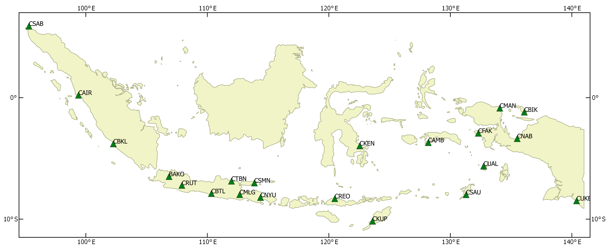
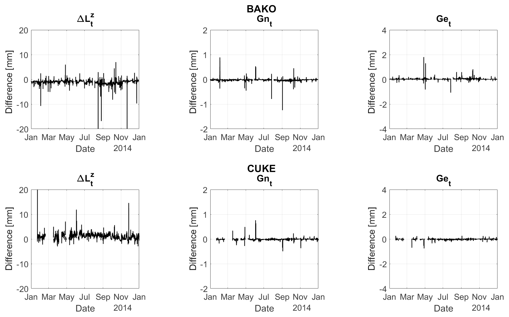
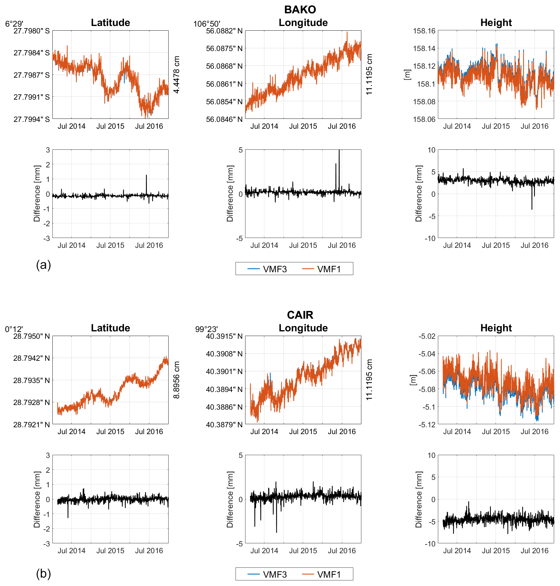
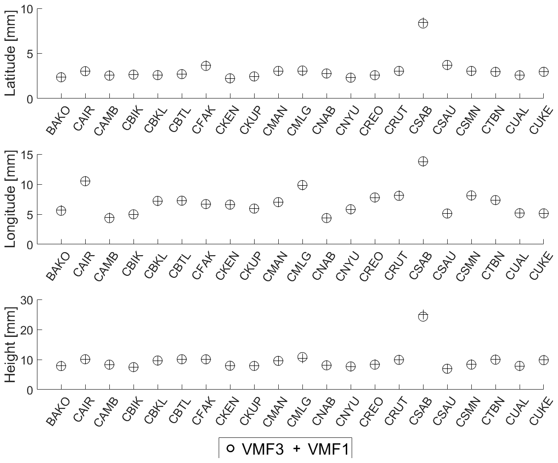
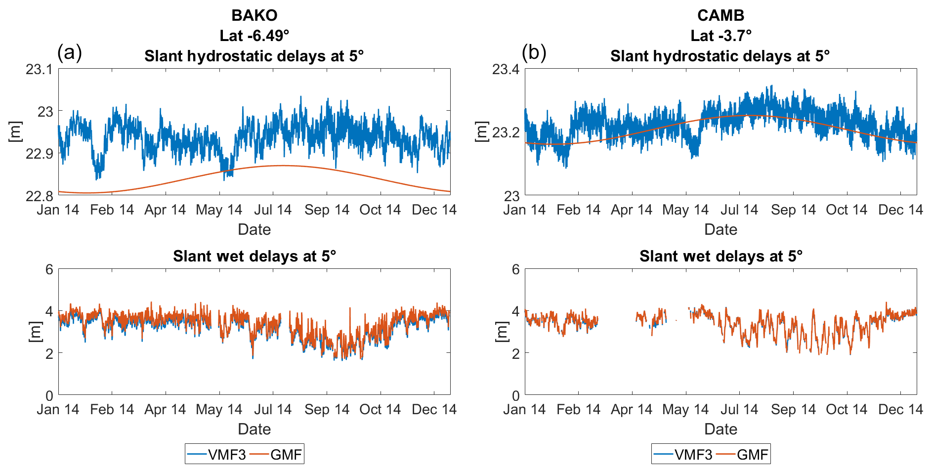
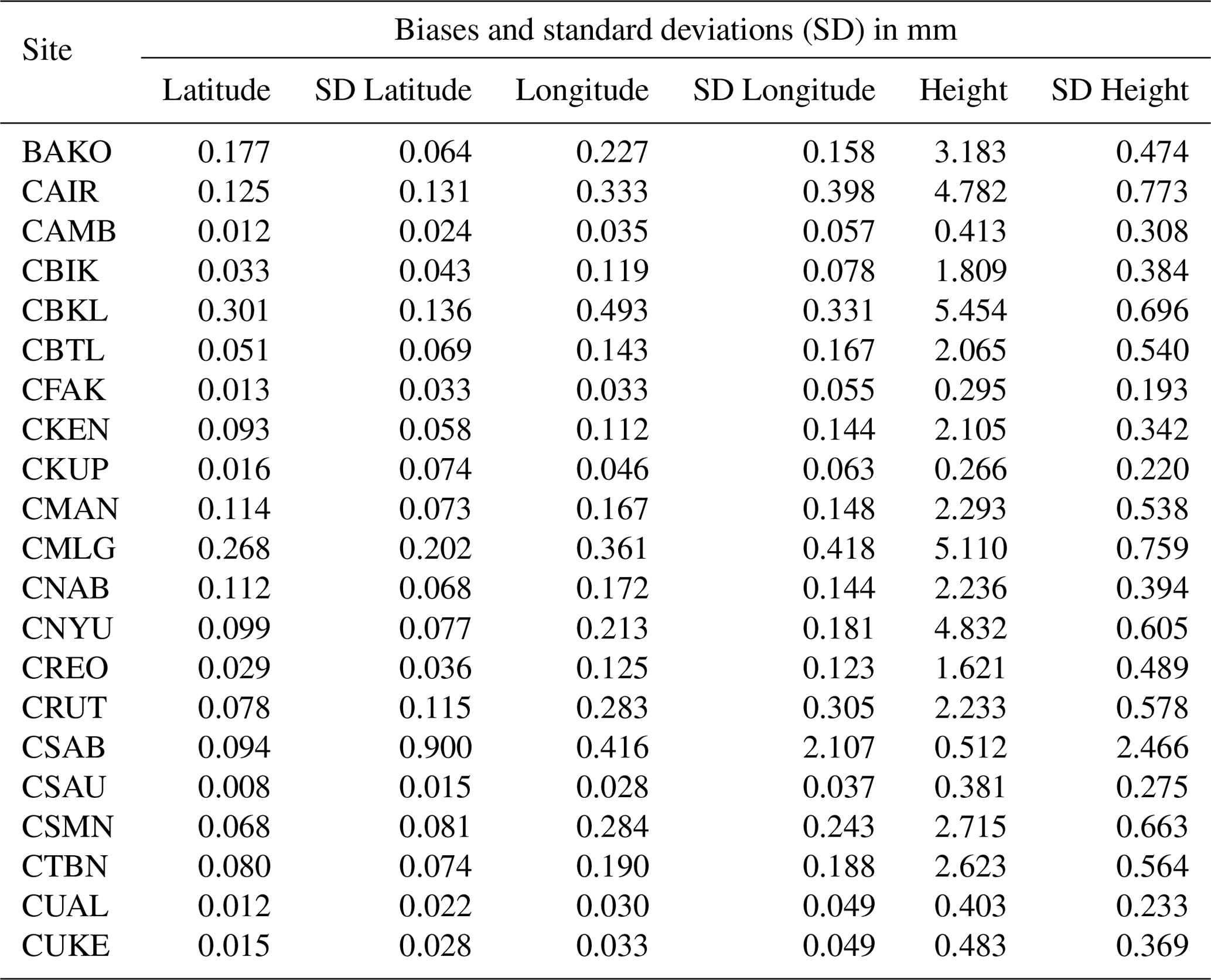
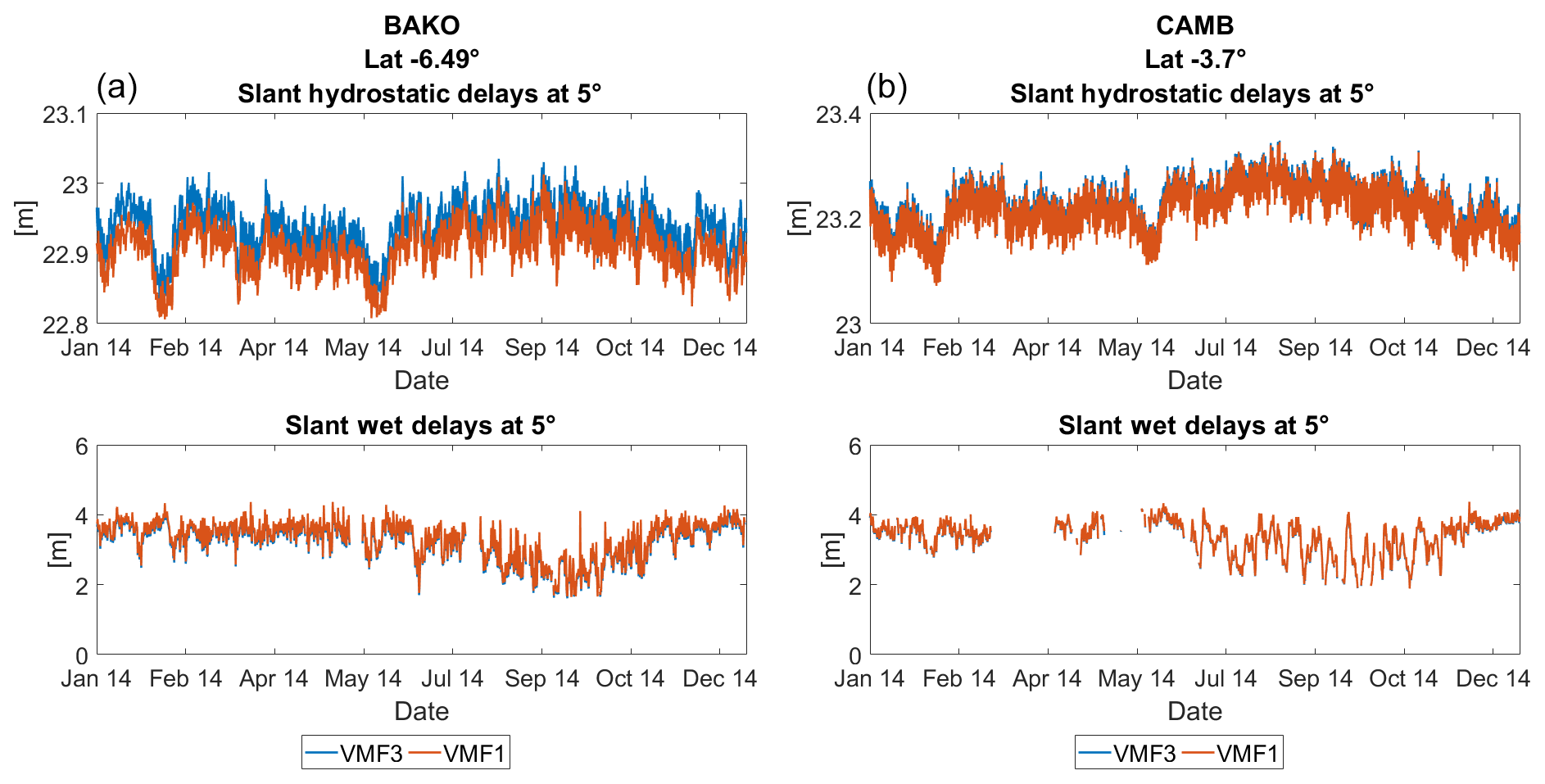
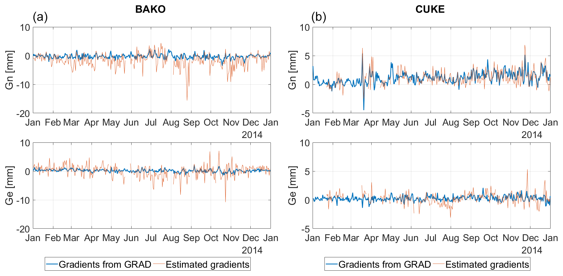
Tropospheric delay is one of the major error sources for space geodetic techniques, such as the Global Navigation Satellite Systems (GNSS). Mapping functions are used to scale the delay from zenith direction to the elevation angle of the signal. Several mapping functions have already been published, including the Global Mapping Functions (GMF) and Vienna Mapping Functions 1 (VMF1). Recently, a refined version of VMF1, VMF3, was released. The tropospheric gradients GRAD were also determined using the same data set as VMF3. This study aims to test the performance of VMF3 on GNSS observations in Indonesia, using observations from 21 stations of the permanent GNSS network in Indonesia, InaCORS. Data processing was carried out using Precise Point Positioning in Bernese GNSS Software, version 5.2 for the year 2014. Station coordinates were estimated daily, while the zenith wet delays were estimated every 30 min and tropospheric gradients were estimated hourly. A similar processing scheme was carried out using GMF and VMF1. Generally, the results from VMF3 agree very well with the results from GMF and VMF1, although small biases can be found, especially for the height component. Based on the repeatability, while there is no significant difference for the latitude and longitude, there are slight improvements for the height, particularly compared to GMF. The estimated gradients tend to fluctuate more compared to gradients from GRAD. The correlation coefficients between the estimated gradients and those from GRAD are small, with the largest being 0.65 at site CUKE.

1 Introduction

Tropospheric delay is one of the major error sources in space geodetic observations. It needs to be taken into account during the analysis to improve the quality of observation model. Generally, tropospheric delays can be divided into two components: the hydrostatic and wet delays. These delays are often described as the delays at the zenith direction.

Zenith hydrostatic delays $\mathrm{\Delta }{L}_{\mathrm{h}}^z$ can be obtained using surface pressure measurements at the station. Several models have been developed to calculate $\mathrm{\Delta }{L}_{\mathrm{h}}^z$, for instance the model by Saastamoinen (1972):

$$\begin{array}{}\text{(1)}& \mathrm{\Delta }{L}_{\mathrm{h}}^z={\displaystyle \frac{\mathrm{0.0022768}\cdot p}{\mathrm{1}-\mathrm{0.00266}\cdot \cos \left(\mathrm{2}\mathit{\phi }\right)-\mathrm{0.28}\cdot {\mathrm{10}}^{-\mathrm{6}}\cdot h_{\mathrm{ell}}}}\end{array}$$

where p is pressure, φ is geographic latitude, and h_ell is ellipsoidal height of the site.

Figure 1 InaCORS stations used in the data analysis.

Zenith wet delays $\mathrm{\Delta }{L}_{\mathrm{w}}^z$ depend on the amount of water vapor in the atmosphere. Since water vapor is highly variable, temporally and spatially, it is more difficult to estimate $\mathrm{\Delta }{L}_{\mathrm{w}}^z$ based only on surface measurements. It is common practice to estimate $\mathrm{\Delta }{L}_{\mathrm{w}}^z$ along with other parameters during the analysis of GNSS observations. Alternatively, it is also possible to approximate $\mathrm{\Delta }{L}_{\mathrm{w}}^z$ using various models, such as using the formula by Askne and Nordius (1987):

$$\begin{array}{}\text{(2)}& \mathrm{\Delta }{L}_{\mathrm{w}}^z={\mathrm{10}}^{-\mathrm{6}}\cdot \left(k_{\mathrm{2}}^{\prime }+{\displaystyle \frac{k_{\mathrm{3}}}{T_{\mathrm{m}}}}\right)\cdot {\displaystyle \frac{R_{\mathrm{d}}\cdot e}{g_{\mathrm{m}}\cdot (\mathit{\lambda }+\mathrm{1})}}\end{array}$$

where $k_{\mathrm{2}}^{\prime }$ and k₃ are empirically determined refractivity constants, R_d is the specific gas constant for dry constituents, and g_m is the mean gravity. This formula requires information on water vapor pressure e, mean temperature weighted with water vapor pressure T_m, and water vapor decrease factor λ.

Mapping functions are then used to scale the tropospheric delays from the zenith direction down to the elevation angle of the signal. Several mapping functions have already been published, for instance the Global Mapping Functions, GMF (Böhm et al., 2006a), and the Vienna Mapping Functions 1, VMF1 (Böhm et al., 2006b). Recently, a refined version of VMF1, VMF3 (Landskron and Böhm, 2017), was released.

VMF3 was developed based on ray-traced delays using data from the European Centre for Medium-Range Weather Forecasts (ECMWF), ERA-Interim, from the year 2001 to 2010, at 3^∘ elevation angle (for $\mathrm{1}{}^{\circ }\times \mathrm{1}{}^{\circ }$ grid) and eight azimuth angles ($\mathrm{0}{}^{\circ }:\mathrm{45}{}^{\circ }:\mathrm{315}{}^{\circ }$). The coefficients a, b, and c were determined using least-squares adjustment. The b and c coefficients have a temporal and spatial dependence, which was accomplished by estimating seasonal fits containing annual and semi-annual terms for the temporal dependence, and using a spherical harmonics expansion up to degree 12 for the spatial dependence.

Tropospheric horizontal gradients also need to be considered to account for azimuthal asymmetry, especially for observations at low elevation angles. Horizontal gradients can be estimated in the analysis of GNSS or Very Long Baseline Interferometry (VLBI) observations. However, it is also possible to obtain these gradients from other sources, such as from Numerical Weather Models (NWMs). The tropospheric gradients GRAD (Landskron and Böhm, 2018) were determined through ray-tracing using the same NWMs as VMF3, based on the model by Chen and Herring (1997):

$$\begin{array}{}\text{(3)}& \mathrm{\Delta }L(\mathit{\alpha },\mathit{\epsilon })=\mathrm{\Delta }{L}_{\mathrm{0}}\left(\mathit{\epsilon }\right)+{\mathrm{mf}}_{\mathrm{g}}\left(\mathit{\epsilon }\right)\cdot [G_{\mathrm{n}}\cdot \cos (\mathit{\alpha })+G_{\mathrm{e}}\cdot \sin (\mathit{\alpha }\left)\right]\end{array}$$

where G_n and G_e are the north and east gradients, respectively, and mf_g is the gradients mapping function. ΔL₀ is the product of the zenith hydrostatic and wet delays with their respective mapping functions (the isotropic part):

$$\begin{array}{}\text{(4)}& \mathrm{\Delta }{L}_{\mathrm{0}}\left(\mathit{\epsilon }\right)=\mathrm{\Delta }{L}_{\mathrm{h}}^z\cdot {\mathrm{mf}}_{\mathrm{h}}\left(\mathit{\epsilon }\right)+\mathrm{\Delta }{L}_{\mathrm{w}}^z\cdot {\mathrm{mf}}_{\mathrm{w}}\left(\mathit{\epsilon }\right)\end{array}$$

This study aims to assess the performance of VMF3 on GNSS observations in Indonesia. For this purpose, 21 stations from the Indonesian permanent GNSS network, InaCORS, were chosen based on their location and data availability. The map of the stations can be seen in Fig. 1. The majority of InaCORS stations are located on Java Island. Most stations on other islands were constructed recently and therefore have limited number of observations.

Data processing was carried out using Precise Point Positioning (PPP) in Bernese GNSS Software 5.2 (Dach et al., 2015) for the year 2014. The elevation cutoff angle is 5^∘, while the antenna corrections, orbit files, and clock corrections are taken from the Center for Orbit Determination in Europe, CODE (Dach et al., 2016). Three different mapping functions were used, namely GMF, VMF1, and VMF3. Since Bernese only supports GMF and VMF1, changes had to be made in the Bernese subroutines in order to allow the software to use VMF3. The codes for VMF3 can be found at http://vmf.geo.tuwien.ac.at/codes/ (last access: 4 March 2020).

Figure 2 Estimated coordinates from VMF3 and GMF and their differences for station BAKO (a) and CAIR (b). On the right side of the latitude and longitude plot, max-min value in cm is given.

Figure 3 The differences of tropospheric parameters from VMF3 and GMF. Zenith wet delays and gradients (north and south) were estimated.

The comparison of estimated coordinates and tropospheric parameters from VMF3 and GMF is shown in Sect. 2, while the comparison with VMF1 is shown in Sect. 3. The slant tropospheric delays at 5^∘ elevation angle from all three mapping functions are shown in Sect. 4. Section 5 presents the comparison of the estimated gradients using VMF3 with the gradients from the model GRAD. Conclusions are drawn in Sect. 6.

2 VMF3 and GMF

The first analysis was carried out using VMF3 troposphere model, specifically the gridded version, since none of the InaCORS stations are part of the IGS network (with the exception of site BAKO). The a priori hydrostatic zenith delays $\mathrm{\Delta }{L}_{\mathrm{h}}^z$ were also taken from the gridded VMF3. Gridded VMF3 is available in two grid sizes: $\mathrm{1}{}^{\circ }\times \mathrm{1}{}^{\circ }$ and $\mathrm{5}{}^{\circ }\times \mathrm{5}{}^{\circ }$ resolutions. For this study, the 1^∘ version was chosen since it has higher resolution than VMF1.

Figure 4 Repeatability of estimated coordinates from VMF3 and GMF.

Figure 5 Estimated coordinates from VMF3 and VMF1 and their differences for station BAKO (a) and CAIR (b). On the right side of the latitude and longitude plot, max-min value in cm is given.

Station coordinates were estimated daily, while zenith wet delays $\mathrm{\Delta }{L}_{\mathrm{w}}^z$ were estimated every 30 min, and tropospheric gradients (both north and east) were estimated hourly. The results were then compared with GMF whose a priori $\mathrm{\Delta }{L}_{\mathrm{h}}^z$ were based on the values of the Global Pressure and Temperature, GPT (Böhm et al., 2007). The estimated coordinates comparison as well as the differences at two stations are shown in Fig. 2, namely at stations BAKO in West Java and CAIR in West Sumatra. BAKO was chosen since it is part of the IGS network, while CAIR since it is located almost at the equator.

Both results, from VMF3 and GMF processing schemes, agree very well at all stations, particularly for the horizontal components. The differences in the estimated latitude and longitude are typically smaller than 1 mm, with the longitude differences slightly larger than the latitude. At some stations, small biases appear in the height component, similar to site CAIR (Fig. 2, lower part). However, in general, the estimated heights from VMF3 and GMF agree well. The differences between the two models for the height component are at the mm level.

Figure 6 The differences of tropospheric parameters from VMF3 and VMF1. Zenith wet delays and gradients (north and south) were estimated.

Figure 7 Repeatability of estimated coordinates from VMF3 and VMF1.

The mean absolute biases and the standard deviations for all 21 sites can be seen in Table 1. For latitude and longitude, the mean biases are smaller than 1 mm, whereas for the height, the mean absolute biases range from less than 1 mm (at station CKUP) to more than 6 mm (at station CBKL).

Table 1 Mean absolute biases and standard deviations for VMF3 and GMF.

Additionally, tropospheric parameters are also compared, namely the zenith total delays $\mathrm{\Delta }{L}_{\mathrm{t}}^z$ and total tropospheric gradients (north and east), Gn_t and Ge_t, respectively. The comparison of the differences between the tropospheric estimates can be seen in Fig. 3. The differences between the estimated $\mathrm{\Delta }{L}_{\mathrm{t}}^z$ from both models are less than 1 cm with a SD of around 0.6 mm. For the estimated gradients, the differences are typically less than 2 mm with a SD of less than 0.1 mm, although the values for Ge_t are larger than Gn_t.

To compare the performance between VMF3 and GMF, the repeatability of the estimated coordinates from each station was determined. The comparison can be seen in Fig. 4. In general, both VMF3 and GMF yield similar results. This is especially true for the horizontal components, latitude and longitude. However, for the height component, using VMF3 yields slightly better results for more than half of the stations, as seen from smaller standard deviations.

Figure 8 Slant hydrostatic and wet delays at 5^∘ from VMF3 and GMF at sites BAKO (a) and CAMB (b).

3 VMF3 and VMF1

The second comparison was done for VMF3 and VMF1, which are both discrete mapping functions. For VMF1, the a priori $\mathrm{\Delta }{L}_{\mathrm{h}}^z$ were taken from the gridded VMF1, which is available for the grid size $\mathrm{2.0}{}^{\circ }\times \mathrm{2.5}{}^{\circ }$. VMF3 and its a priori $\mathrm{\Delta }{L}_{\mathrm{h}}^z$ were taken from the $\mathrm{1}{}^{\circ }\times \mathrm{1}{}^{\circ }$ grid size, similar to Sect. 2.

The comparison of estimated coordinates and their differences at sites BAKO and CAIR can be seen in Fig. 5. The differences between VMF3-VMF1 are generally smaller than VMF3-GMF at all sites, probably because both are discrete mapping functions, whereas GMF is empirical. Small biases of a few mm also appear in the height component, as with GMF, only to a smaller degree.

The mean absolute biases and the standard deviations can be seen in Table 2. Compared to GMF, the biases for VMF1 are generally smaller. This is especially obvious for the height component.

Table 2 Mean absolute biases and standard deviations for VMF3 and VMF1.

The differences in tropospheric estimates ($\mathrm{\Delta }{L}_{\mathrm{t}}^z$, Gn_t, and Ge_t) can be seen in Fig. 6. The results are quite similar as the differences between tropospheric estimates from VMF3-GMF.

Figure 9 Slant hydrostatic and wet delays at 5^∘ from VMF3 and VMF1 at sites BAKO and CAMB.

Figure 10 Comparison of gradients from GRAD with the estimated gradients at site BAKO and CUKE.

The repeatability of the estimated coordinates from VMF3 and VMF1 are depicted in Fig. 7. The results from VMF3 and VMF1 are very similar for all three components. The height components at some sites are slightly improved when using VMF3.

4 Slant delays at 5^∘

Slant delays at 5^∘ were calculated using VMF3, VMF1, and GMF. In the case of VMF3 and VMF1, a priori zenith hydrostatic delay $\mathrm{\Delta }{L}_{\mathrm{h}}^z$ was based on the ECMWF re-analysis data using Eq. (1). For GMF, a priori $\mathrm{\Delta }{L}_{\mathrm{h}}^z$ was computed based on the values from the Global Pressure and Temperature, GPT (Böhm et al., 2007).

The comparison of slant delays at two sites from VMF3 and GMF can be seen in Fig. 8. While a seasonal pattern is clear for ΔL_h from GMF, such pattern is not very visible in the case of VMF3 for most sites. However, the seasonal pattern is more visible for the estimated slant wet delays ΔL_w. This might be due to the fact that Indonesia's climate is mainly characterized by changes in rainfall, instead of temperature and pressure. The variation in rainfall is due to the monsoon patterns, whose changes in directions correspond to the dry season and the rainy season. For regions located in the south of equator, the dry season occurs from June to October and rainy season from November to March. For regions located in the north of equator, the opposite is the case. Closer to the equator, the amount of rainfall throughout the year does not vary significantly.

ΔL_h at site BAKO from GMF is smaller than from VMF3 (Fig. 8, left side). This is also the case at some other sites. However, for most other sites, including site CAMB (Fig. 8, right side), ΔL_h from VMF3 agrees well with ΔL_h from GMF.

Seasonal patterns can be seen in ΔL_w for sites BAKO. ΔL_w is smaller between May and November, which coincides with the middle of the dry season until the beginning of the rainy season in Indonesia. Generally, seasonal patterns are more obvious at sites located farther away from the equator. However, for sites located in the eastern part of Indonesia, in Papua and on the islands of Maluku (e.g. site CAMB), the seasonal pattern for ΔL_w is not visible.

The comparison of slant delays from VMF3 and VMF1 are depicted in Fig. 9. Biases can be seen for the ΔL_h at sites BAKO and several other sites. These biases seem to correlate with the bias from GMF, suggesting that the biases come from VMF3.

5 Comparison with gradients from GRAD

The estimated gradients as obtained from the analysis of GNSS observations are compared with the gradients from the model GRAD. Comparison at two sites, BAKO and CUKE can be seen in Fig. 10. The estimated gradients have larger magnitude compared to gradients from GRAD.

The correlation coefficients for G_n and G_e at site BAKO are 0.41 and 0.33, respectively. The values are similar for the other sites, with the values G_n tending to be larger than G_e. The largest value for G_n is 0.65 at site CUKE, while the largest G_e value is 0.41 at site CNAB, both are located in Papua.

Low correlation coefficients mean that the estimated gradients do not fit well with the gradients from GRAD. The estimated gradients are noisier, possibly because GRAD was determined using NWMs, which are already smoothed. During GNSS data processing, other parameters were also estimated and this might introduce some errors in the results. Gradients are also sensitive to the processing settings, such as the elevation cutoff angle, gradient mapping function, and GNSS constellation, as shown by Kačmařík et al. (2019).

6 Conclusions

While there are no significant improvements in latitude and longitude, applying VMF3 together with its hydrostatic zenith delays can improve the height component compared to GMF/GPT, as seen from the repeatability. However, in comparison with VMF1, only a slight improvement in the height component can be seen.

Biases at some sites can be seen in the slant hydrostatic delays at 5^∘ between VMF3 and both VMF1 and GMF. The estimated gradients are noisier compared to the gradients from the model GRAD, possibly due to the fact that GRAD was determined using smoothed NWMs and errors are introduced during the GNSS processing which can affect the estimated gradient parameters.

It is recommended to use NWM-based mapping functions, such as VMF3 and VMF1. However, considering that the performance of VMF3 is comparable to VMF1, at this point we cannot conclusively recommend using VMF3 in place of VMF1 for GNSS stations in Indonesia.

References

Askne, J. and Nordius, H.: Estimation of tropospheric delay for microwaves from surface weather data, Radio Sci., 22, 379–386, 1987. a
Böhm, J.: Index of /trop_products, available at: https://vmf.geo.tuwien.ac.at/trop_products/, last access: 4 March 2020. a
Böhm, J., Niell, A., Tregoning, P., and Schuh, H.: Global Mapping Function (GMF): A new empirical mapping function based on numerical weather model data, Geophys. Res. Lett., 33, L07304, https://doi.org/10.1029/2005GL025546, 2006a. a
Böhm, J., Werl, B., and Schuh, H.: Troposphere mapping functions for GPS and VLBI from ECMWF operational analysis data, J. Geophys. Res, 111, B02406, https://doi.org/10.1029/2005JB003629, 2006b. a
Böhm, J., Heinkelmann, R., and Schuh, H.: Short note: a global model of pressure and temperature for geodetic applications, J. Geodesy, 81, 679–683, 2007.  a, b
Chen, G. and Herring, T.: Effects of atmospheric azimuthal asymmetry on the analysis of space geodetic data, J. Geophys. Res.-Sol. Ea., 102, 20489–20502, 1997. a
Dach, R., Lutz, S., Walser, P., and Fridez, P. (Eds.): Bernese GNSS Software Version 5.2. User manual, Astronomical Institute, University of Bern, Bern Open Publishing, 2015. a
Dach, R., Schaer, S., Arnold, D., Orliac, E., Prange, L., Susnik, A., Villiger, A., and Jäggi, A.: CODE final product series for the IGS, available at: http://ftp.aiub.unibe.ch/CODE/ (last access: 4 March 2020), 2016. a
Kačmařík, M., Douša, J., Zus, F., Václavovic, P., Balidakis, K., Dick, G., and Wickert, J.: Sensitivity of GNSS tropospheric gradients to processing options, Ann. Geophys., 37, 429–446, https://doi.org/10.5194/angeo-37-429-2019, 2019. a
Landskron, D. and Böhm, J.: VMF3/GPT3: refined discrete and empirical troposphere mapping functions, J. Geodesy, 92, 349–360, 2017. a
Landskron, D. and Böhm, J.: Refined discrete and empirical horizontal gradients in VLBI analysis, J. Geodesy, 92, 1387–1399, https://doi.org/10.1007/s00190-018-1127-1, 2018. a
Saastamoinen, J.: Atmospheric correction for the troposphere and stratosphere in radio ranging of satellites. In: Henriksen SW et al. (eds) The use of artificial satellites for geodesy, vol 15. AGU, Washington, 247–251, 1972. a
Download
Short summary
Tropospheric delays must be taken into account when analyzing GNSS data. Several tropospheric delay models and mapping functions are available, for instance the Vienna Mapping Functions 1 (VMF1) and the Global Mapping Function (GMF). Recently, a refined version of VMF1, VMF3, has been released. This study aims to assess the performance of VMF3 for GNSS observations in Indonesia, by analyzing the data using Bernese GNSS Software, version 5.2 with Precise Point Positioning method.