 | 07 Aug 2019
Comparing atmospheric data and models at station Wettzell during CONT17
Daniel Landskron
Johannes Böhm
Thomas Klügel
Torben Schüler
During the Continuous Very Long Baseline Interferometry (VLBI) Campaign 2017 (CONT17), carried out from 28 November through 12 December 2017, an extensive data set of atmospheric observations was acquired at the Geodetic Observatory Wettzell. In addition to in situ measurements of temperature, humidity, pressure or wind speed at the surface, radiosonde ascents yielded meteorological parameters continually up to 25 km height, and integrated water vapor (IWV) was obtained at several elevations and azimuths from a water vapor radiometer. Troposphere delays estimated from Global Navigation Satellite Systems (GNSS) observations plus comparative values from two different Numerical Weather Models (NWMs) complete the abundance of data. In this presentation, we compare these data sets to parameters of the Vienna Mapping Functions 1 and 3 (VMF1 & VMF3), which are based on NWM data by the ECMWF, and to estimates of VLBI analysis using the Vienna VLBI and Satellite Software (VieVS). On the one hand, we contrast the variety of troposphere delays in zenith direction with each other, while on the other hand we utilize radiosonde data and meteorological observations at the site to create local mapping functions which can then be compared to VMF3 and VMF1 at Wettzell. In general, we thus received very good accordance between the different solutions. Also in terms of the mapping functions, the local radiosonde mapping function is in consistence with VMF1 and VMF3 with differences less than 5 mm at 5∘ elevation.
- Article
(497 KB) - Full-text XML
- BibTeX
- EndNote


From 28 November through 12 December 2017, the Geodetic Observatory Wettzell carried out an extensive measurement campaign of atmospheric and meteorological parameters (Klügel et al., 2019). The time frame was actually chosen such as to coincide with CONT17, the Continuous VLBI (Very Long Baseline Interferometry) experiment 2017. Beside a number of further data such as wind speed, cloud coverage or solar radiation, the following observations are of importance for the present study:
-
a local meteo station measured pressure, temperature and humidity at the surface every minute
-
a water vapor radiometer determined the integrated water vapor (IWV) of the air at several elevation and azimuth angles every minute
-
semi-daily ascents of radiosondes built vertical profiles of pressure, temperature and humidity up to 25 km height
-
two independent Global Navigation Satellite Systems (GNSS) analyses yielded hourly zenith total delays ΔLz at station WTZR, once performed by BKG data center (GNSSBKG) and once performed by the Wettzell local array using the inhouse analysis software SGSS (GNSSWETT) (Klügel et al., 2019).
In addition to this observation campaign, we supplement the data sets with the following quantities:
-
hourly zenith wet delays estimated from VLBI analysis at the station WETTZELL using the Vienna VLBI and Satellite Software (VieVS; Böhm et al., 2018)
-
six-hourly zenith hydrostatic delays and zenith wet delays from Numerical Weather Model (NWM) data by NCEP (National Center for Environmental Prediction)
-
six-hourly zenith hydrostatic delays , zenith wet delays and mapping factors mfh and mfw from the Vienna Mapping Functions 3 (VMF3; Landskron and Böhm, 2017). VMF3 is determined by 2-D-ray-tracing through NWM data by the ECMWF (European Centre for Medium-range Weather Forecasts) in horizontal resolution and 25 pressure levels.
-
six-hourly zenith hydrostatic delays , zenith wet delays and mapping factors mfh and mfw from the Vienna Mapping Functions 1 (VMF1; Böhm et al., 2006). VMF1 is determined by 1-D-ray-tracing through NWM data by the ECMWF in horizontal resolution and 21 pressure levels.
The resulting wealth of data enables an extensive comparison of the different quantities and allows inferences about the performances of the different observation techniques.
The upcoming Sect. 2 enumerates the preparatory work that had to be done prior to the data analysis. Section 3 outlines the necessary steps for deriving a mapping function from radiosonde data. Section 4 elaborates on the results of the various comparisons, before the findings are concluded in Sect. 5.
For ensuring full consistency, the observations had to be treated ahead of the comparison. This treatment mainly encompasses the reduction to a uniform height level and the temporal interpolation.
2.1 Height reductions
The various observations are each valid for different heights. The radiosondes were launched from the surface, the pressure sensor is located inside a building, the GNSS antenna is mounted on the roof of a building, while the reference point of the VLBI antenna is located some 20 m above the ground. As a rule of thumb, a height difference of 8 m corresponds to a pressure difference of approximately 1 hPa, which in further consequence causes a difference in zenith hydrostatic delay of 2.5 mm. Hence, non-consideration of a uniform height level would introduce significant biases into the comparison. We therefore define the ellipsoidal reference height hell as 666 m, which is in fact the height of the GNSS antenna, and reduced all data to this height.
For the reduction of the zenith hydrostatic delay , we applied Eqs. (1)–(3) as suggested by Kouba (2008). The index 0 here denotes the original height of the observation, whereas h means the ellipsoidal reference height of 666 m. Additionally, φ is the geographic latitude.
That is, is first converted to the respective pressure value. This pressure is then reduced to the reference height and converted back to zenith hydrostatic delay.
The zenith wet delay does not decrease linearly with height and may be subject to several inversions, therefore the reduction in Eq. (4) is only an approximation (Kouba, 2008).
Lastly, also the hydrostatic mapping function mfh, whose creation is outlined in the upcoming Sect. 3, requires a height reduction. For this purpose, we follow the reduction by Niell (1996) (Eq. 5). The elevation angle of the observation is denoted with ε here.
Inaccuracies resulting from the height reductions, however, bear the risk of introducing biases to the comparisons. There is no necessity for any horizontal reductions, as all measuring sites in Wettzell are located in immediate vicinity.
2.2 Temporal interpolation
To overcome the problem of different temporal resolutions, interpolations were made. As the radiosondes were launched only twice daily, we interpolated the other data to these reference epochs using spline interpolation.
2.3 Further preparations
The water vapor radiometer outputs IWV, which has to be converted to zenith wet delay prior to the comparison. This is handled with Eq. (6) as suggested by Askne and Nordius (1987).
Here, k2′ and k3 are empirical constants, Tm is the weighted mean temperature of water vapor pressure and Rw is the specific gas constant of water vapor.
Moreover, in order to derive the GNSS zenith wet delay , the zenith hydrostatic delay from the in situ pressure measurements was subtracted from the GNSS zenith total delay ΔLz.
All mapping functions by TU Wien such as VMF3 and VMF1 are based on ray-tracing through NWMs. This has the big advantage that they are valid for the whole Earth and in a temporal resolution of four times a day. A drawback is, however, the comparably small vertical resolution of 25 pressure levels from 1000 to 1 hPa, which can only be further densified through interpolation. Radiosondes can overcome this problem as they profile the entire atmosphere above the station very densely. On their way from the surface to their maximum height at up to 25 km (the point where the balloons burst), radiosondes measure temperature, pressure and humidity every second, thus yielding a vertical resolution of up to 5000 levels.
For processing the radiosonde data, it was first necessary to convert temperature T and humidity r in [%] to water vapor pressure e, which was accomplished with the Magnus formula in Eq. (7).
With this, the hydrostatic refractivity Nh and wet refractivity Nw at each layer can be determined using Eqs. (8) and (9).
Integrating these refractivities over the full height range directly yields and , respectively.
The determination of mapping functions from radiosonde data is not as straightforward, though. Here, the path delays are not only required in zenith direction, but also in slant elevation angles. The radiosonde profile is only 1-D, that is, there is no information about the horizontal distribution of the meteorological quantities. It is therefore necessary to proceed on the simplified assumption that the vertical radiosonde profile is valid also in the vicinity of the station. The atmosphere can thus be imagined as a series of plates stacked over one another. For high elevation angles, this simplification is certainly unproblematic. For very low elevation angles, however, it may have a negative impact on the accuracy.
The ray-tracing technique applied here is referred to as 1-D-ray-tracing, that is, the constructed ray path is subject to refractivity changes only in one dimension. This technique is also utilized for VMF1. In contrast, for VMF3 a 2-D-ray-tracer is used, which considers also horizontal changes in refractivity. For the sake of completeness, it should be mentioned that in 3-D-ray-tracing the ray path would additionally not be fixed to a vertical, two-dimensional plane, but would propagate like a space curve.
The ray-tracing yields zenith delays as well as mapping factors at the elevation angle 3∘. Different azimuth angles are not necessary, as the 1-D distribution of the atmospheric profile would not make any difference with azimuth anyway. In order to make the mapping available for arbitrary elevation angles, the mapping factors must be converted into the mapping function coefficients a, b and c. This is done using the empirical representations of b and c from VMF3 and thus calculating the a coefficients by means of inverting Eq. (10) by Marini (1972).
The resulting local radiosonde mapping function can thus be used just like VMF3 and VMF1.
The comparisons are done for zenith hydrostatic delays , zenith wet delays and for mapped slant hydrostatic delays ΔLh and slant wet delays ΔLw at an elevation angle of 5∘.
4.1 Zenith delays
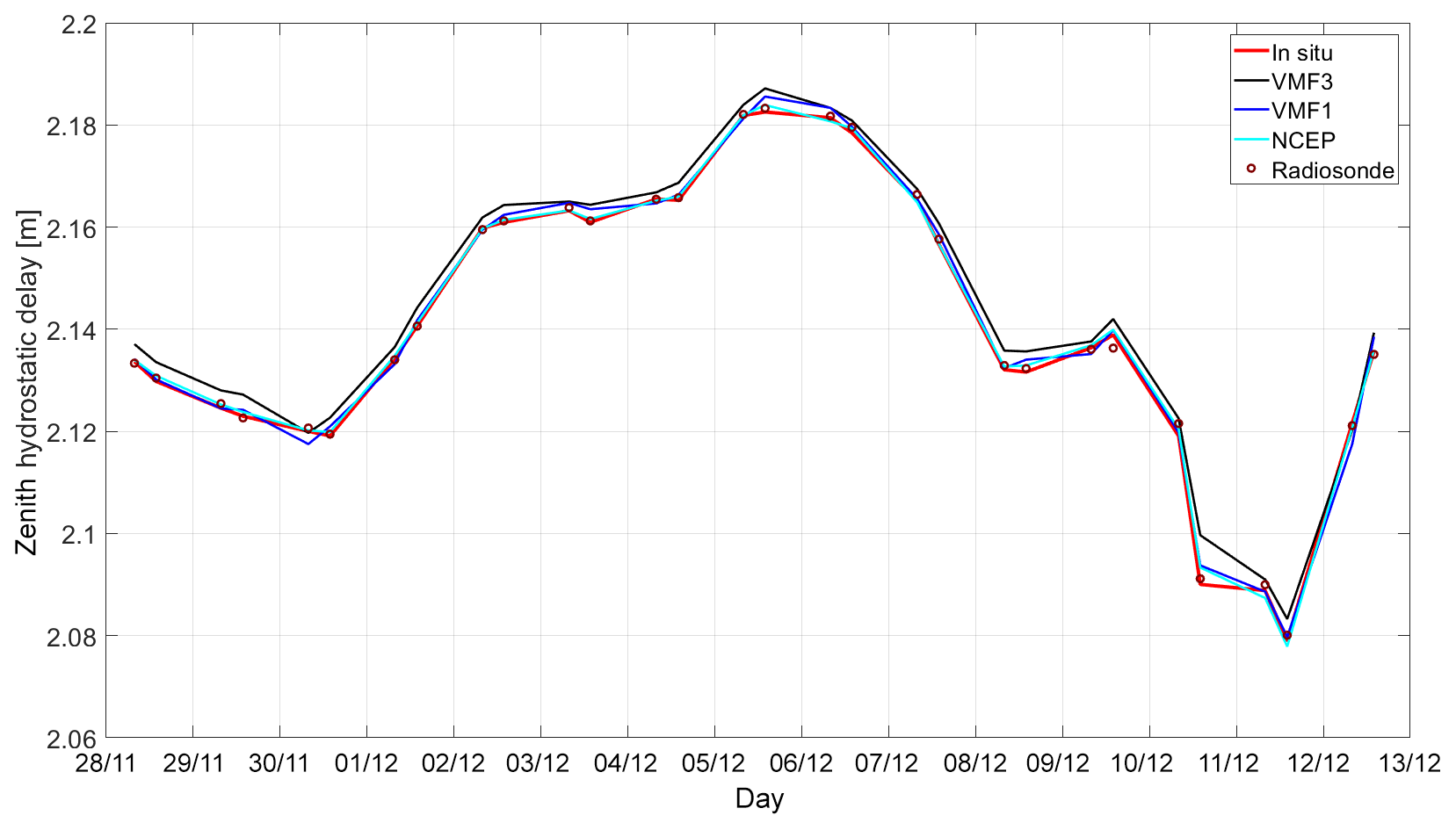
Figure 1 shows that all zenith hydrostatic delays fit together very well. The ones from in situ pressure measurements are regarded as the most accurate representation, so they serve as reference values in Table 1.
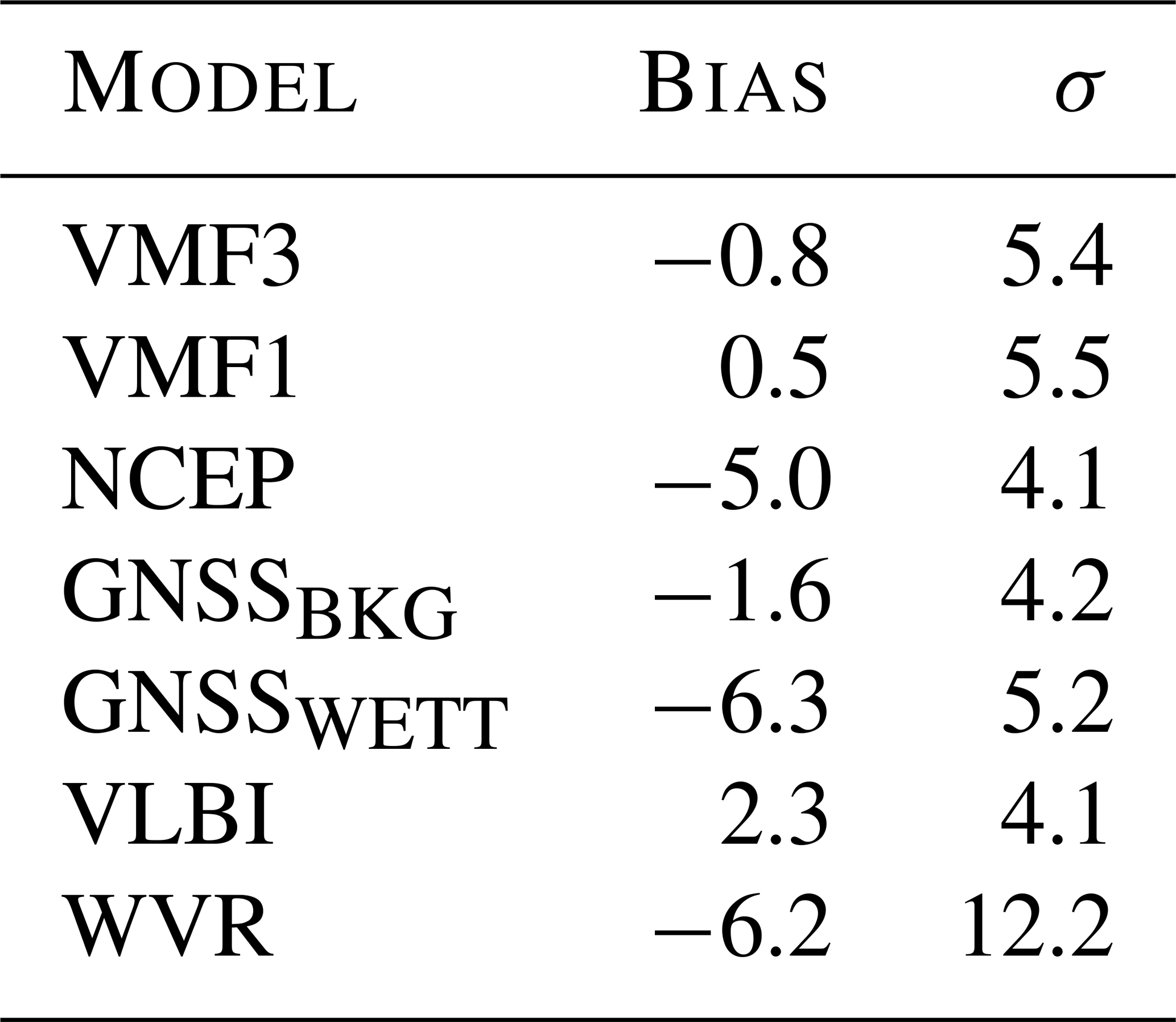
Table 1Bias and standard deviation in zenith hydrostatic delay (mm) between the reference solution from in situ pressure measurements and the other solutions.

The zenith hydrostatic delays from NCEP and from the radiosondes fit best, whereas there appears to be a small bias in the zenith hydrostatic delays from VMF3. However, since an inaccuracy in station height of 3 m would be reflected in a zenith hydrostatic delay difference of approximately 1 mm, these numbers have to be treated with caution. Another reason for differences are the different horizontal resolutions of the NWMs. For NCEP and VMF3, the horizontal resolution is . VMF1, on the other hand, is determined from NWMs. As a result, we do not see differences in the low millimeter range as to be effective.

As was expected, the accordance in zenith wet delay is not as high as in (cf. Fig. 2), since the wet part of the delay is usually more fluctuating than the hydrostatic part. This is also reflected in Table 2, where all solutions are referenced to that of the radiosondes, which is expected to be the most precise one.
Table 2Bias and standard deviation in zenith wet delay (mm) between the reference solution from radiosonde data and the other solutions.
Water vapor radiometers are known to be error-prone in periods of rain, as thus the lens of the radiometer can be covered with water. Also the WVR used in this analysis yielded occasional unrealistically high values, which were excluded using the 3⋅σ criterion. However, the two outliers on 4 and 11 December appear to have slipped through this exclusion. Most likely, the outliers stem from rain periods, which is confirmed by comparison with rain measurements in Klügel et al. (2019).
4.2 Slant delays
For the comparison of slant delays, the delays from radiosonde data are again used as reference values. As they are, in contrast to VMF3 and VMF1, determined from direct measurements of the atmospheric situation above the site, they are expected to be of high quality. Nevertheless, there are some limitations and drawbacks of the radiosonde data:
-
The radiosonde profile is processed as if it were strictly vertical. In reality, however, radiosondes do not ascend vertically, but are moved by winds, especially by trade winds in higher altitudes. The radiosondes used in this study traveled up to 150 km eastwards before bursting at an altitude of 20–25 km. Thus, the measured profile is in fact not vertical, but is inclined at an elevation angle of approximately 15∘ from the station.
-
The radiosonde profiles are only one-dimensional. When ray-tracing especially at low elevation angles, the resulting mapping functions thus do not reflect the real atmospheric situation around the site.
-
The radiosondes ascend for up to 90 min in order to reach their maximum height, but the integrated zenith delays and mapping functions are each valid for launch time.
-
The current height of a radiosonde is constantly measured with absolute GNSS positioning, which generally has an accuracy in the low meter range. As described in Sect. 4.1, this may impact the resulting zenith delays.
Figure 3 and Table 3 describe the differences in slant hydrostatic delay.

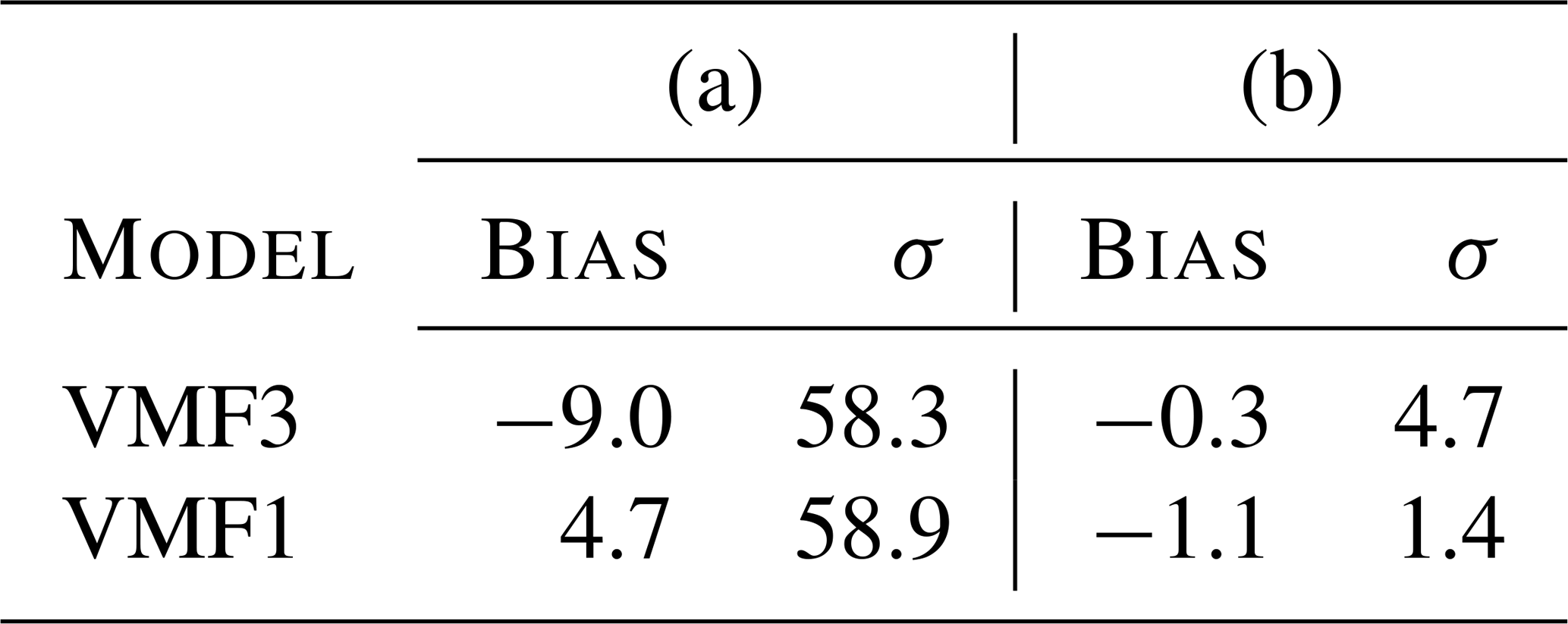
Table 3Bias and standard deviation in slant hydrostatic delay ΔLh (mm) at 5∘ elevation between the reference solution from radiosonde data and the other solutions. In the left part of the table (a), the zenith delays as well as the mapping functions come from the respective model; in the right part (b), the zenith delays from the radiosonde data are used for all models, so that the results reflect only the difference in mapping functions.

There is a noticeably high bias in VMF3 in part (a), which however stems mostly from the bias in (see Table 1). The standard deviations are fairly equal. Part (b) proves that the differences in the mapping factors are negligibly small, that is, the differences come mainly from the zenith delays. For the sake of completeness it is mentioned again that VMF1 is determined with a 1-D ray-tracer, just like the radiosonde data, which might cause correlations in the solutions.
Lastly, Fig. 4 and Table 4 illustrate the difference in slant wet delay ΔLw, again with the radiosonde data being the reference solution.
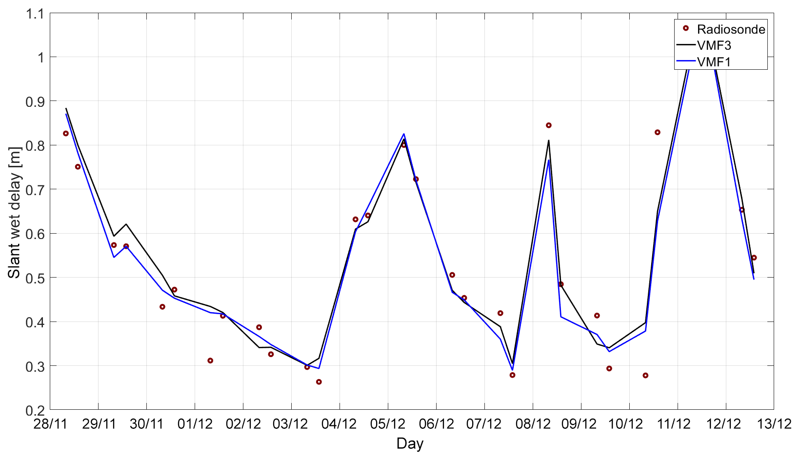
Table 4Bias and standard deviation in slant wet delay ΔLw (mm) at 5∘ elevation between the reference solution from radiosonde data and the other solutions. In the left part of the table (a), the zenith delays as well as the mapping functions come from the respective model; in the right part (b), the zenith delays from the radiosonde data are used for all models, so that the results reflect only the difference in mapping functions.
The radiosonde delays are significantly farther away from the VMF delays here. Also there is a higher bias in VMF3 than in VMF1, which comes again from the zenith delays. Apart from that, the mapping factors from VMF3 appear to fluctuate more than those of VMF1, although their bias is smaller. These differences are in a fairly small range, though. In general, it is very pleasant that the differences resulting only from the mapping functions (column (b) in Tables 3 and 4) are at or below 5 mm. According to a rule of thumb by Böhm (2004), an error of 5 mm in slant delay at 5∘ elevation corresponds to an error in station height of 1 mm.
In this paper, we have compared meteorological data sets from the Geodetic Observatory Wettzell with data from VMF3 and VMF1 as well as with estimates from GNSS and VLBI analyses. The main outcome is that in principle all solutions are in good accordance with each other. All techniques capture the same medium-term weather changes as well as most short-term weather changes. The zenith wet delays estimated in GNSS and VLBI analyses agree very well with each other and with other solutions, although the Wettzell in-house solution GNSSWETT performs slightly worse than the GNSS solution by BKG. On the other hand, the hydrostatic delays from VMF3 seem to be systematically larger than those of the reference solutions. However, it cannot be ruled out that these biases come (partly) from inaccuracies in the specified heights. In terms of slant delays it is shown that the local mapping function derived from radiosonde data yields very similar results as VMF3 and VMF1. The differences in slant delay at 5∘ elevation resulting from the different mapping functions amount to 5 mm at maximum, which corresponds to a station height error of only 1 mm. Also here it has to be noted that there are several accuracy-limiting factors in the genesis of the mapping functions, which is why we do not regard small differences as to be effective.
The meteorological data sets by the Wettzell Geodetic Observatory are available at https://doi.pangaea.de/10.1594/PANGAEA.895518 (Klügel et al., 2018), while the VMF3 and VMF1 data can be downloaded at http://vmf.geo.tuwien.ac.at.
DL carried out the data analysis for the comparison. TK and TS were in charge of the creation of the Wettzell meteorological data sets, while DL and JB generated the VMF3, VMF1 and VLBI data sets. DL prepared the manuscript with contributions from all co-authors.
The authors declare that they have no conflict of interests.
This article is part of the special issue “European Geosciences Union General Assembly 2019, EGU Geodesy Division Sessions G1.1, G2.4, G2.6, G3.1, G4.4, and G5.2”. It is a result of the EGU General Assembly 2019, Vienna, Austria, 7–12 April 2019.
This research has been supported by the FWF Der Wissenschaftsfonds (RADIATE ORD project (ORD 68 Open Research Data)).
This paper was edited by Holger Steffen and reviewed by two anonymous referees.
Askne, J. and Nordius, H.: Estimation of tropospheric delay for microwaves from surface weather data, Radio Sci., 22, 379–386, 1987. a
Böhm, J.: Troposphärische Laufzeitverzögerungen in der VLBI, Veröffentlichung des Institutes für Geodaesie und Geophysik, Geowissenschaftliche Mitteilungen, Heft Nr. 68, ISSN 1811-8380, 2004 (in German). a
Böhm, J., Werl, B., and Schuh, H.: Troposphere mapping functions for GPS and VLBI from European Centre for Medium-Range Weather Forecasts operational analysis data, J. Geophys. Res., 111, B02406, https://doi.org/10.1029/2005JB003629, 2006. a
Böhm, J., Böhm, S., Boisits, J., Girdiuk, A., Gruber, J., Hellerschmied, A., Krasna, H., Landskron, D., Madzak, M., Mayer, D., McCallum, J., McCallum, J., Schartner, M., and Teke, K.: Vienna VLBI and Satellite Software (VieVS) for Geodesy and Astrometry, Publ. Astron. Soc. Pac., 130, 986, https://doi.org/10.1088/1538-3873/aaa22b, 2018. a
Klügel, T., Böer, A., Schüler, T., and Schwarz, W.: Atmospheric measurements from the Geodetic Observatory Wettzell during the CONT-17 VLBI campaign (November 2017–December 2017), PANGAEA, https://doi.org/10.1594/PANGAEA.895518, 2018. a
Klügel, T., Böer, A., Schüler, T., and Schwarz, W.: Atmospheric data set from the Geodetic Observatory Wettzell during the CONT-17 VLBI campaign, Earth Syst. Sci. Data, 11, 341–353, https://doi.org/10.5194/essd-11-341-2019, 2019. a, b, c
Kouba, J.: Implementation and testing of the gridded Vienna Mapping Function 1 (VMF1), J. Geodesy, 82, 193–205, https://doi.org/10.1007/s00190-007-0170-0, 2008. a, b
Landskron, D. and Böhm, J.: VMF3/GPT3: refined discrete and empirical troposphere mapping functions, J. Geodesy, 92, 349–360, https://doi.org/10.1007/s00190-017-1066-2, 2017. a
Marini, J. W.: Correction of satellite tracking data for an arbitrary tropospheric profile, Radio Sci., 7, 223–231, 1972. a
Niell, A. E.: Global mapping functions for the atmosphere delay at radio wavelengths, J. Geophys. Res., 101, 3227–3246, 1996. a