 | 14 Sep 2018
A methodology for optimizing probabilistic wind power forecasting
Christos Stathopoulos
George Galanis
Nikolaos S. Bartsotas
Deterministic wind power forecasts enclose an inherent uncertainty due to several sources of error. In order to counterbalance this deficiency, an analysis of the error characteristics and construction of probabilistic forecasts with associated confidence levels is necessary for the quantification of the corresponding uncertainty. This work proposes a probabilistic forecasting method using an atmospheric model, optimization techniques for addressing the temporal error dependencies and Kalman filtering for eliminating systematic errors and enhancing the symmetry-normality of the shaped error distributions. The method is applied in case studies, using real time data from four wind farms in Greece. The performance is compared against a reference method as well as other common methods showing an improvement in the predictive reliability.
- Article
(2462 KB) - Full-text XML
- BibTeX
- EndNote


During recent years, a substantial amount of energy stems from renewable applications, including wind farms of significant spatial extent. Information regarding the forthcoming generated energy can benefit management strategies for the increase of the energy penetration index as well as the prevention of instabilities that result to financial losses.
In relation to wind power forecasting, several scientific and technical approaches have been proposed, contributing to the reduction of the estimated error of the energy yield (Jung and Broadwater, 2014). Likewise, wind power forecasts mostly incorporate the assessment of wind speed, a meteorological variable inherently uncertain with intense variability. As a result, discrepancies between actual and prognostic values are inevitable in cases of deterministic predictions, especially over areas with complex topography.
A way to counterbalance this shortcoming lies in the provision of a range of values, within which the observation is expected to occur. This involves confidence intervals (CI) and quantification of the corresponding uncertainty for the forthcoming examined value and is defined as probabilistic forecast. This approach addresses specific drawbacks, such as the error of deterministic forecasts, rapid alterations in observations, inadequate system response and extreme values. Additionally, prediction intervals can be utilized by energy operators not only for decision-making purposes, but also as a way of evaluating the reliability of deterministic forecasts.
A common practice for the construction of prediction intervals is the formation of theoretical or custom distributions derived from the deterministic prediction errors and the generation of conditional interval forecasts. A range of forecasts can also be obtained by ensemble forecasting outputs from Numerical Weather Prediction (NWP) models with different initializations or physical parameterizations and the further conversion into energy potential (Pinson et al., 2009).
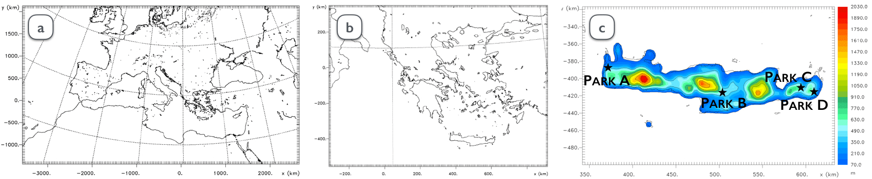
Figure 1(a) Coarse model domain of 36×36 km resolution, (b) 1st nested domain of 6×6 km resolution and (c) 2nd nested domain of 3×3 km resolution, together with parks position of nominal power (from left to right) 9, 5, 5.5 and 12 MW.
Statistical methods for the construction of prediction intervals are briefly summarized in two main categories: (i) the parametric approaches that are linked to a certain distribution and (ii) the non-parametric that assume empirical distributions without restrains for adaptation to specific ones (Tastu et al., 2014).
This work focuses on the estimation of wind power production intervals using a NWP model and taking into account the uncertainty enclosed in the prediction of wind speed and wind power. The development of the probabilistic forecasting methodology is based on key features of the deterministic prediction error. More precisely, it exploits information deriving from error characteristics in terms of discrete counterparts and repeatability. Furthermore, the method relies on the formation of error distributions stemming from the application of a non-linear Kalman filter in different quantiles of the power curve. The proposed methodology is applied to a number of wind power farms and the efficiency is examined through statistical indexes of performance for probabilistic forecasting and comparison against other common methods.
Forecasted meteorological parameters are provided by the high-resolution integrated atmospheric model RAMS/ICLAMS (Fig. 1). The core of the model is based on the limited-area model RAMS6.0 (Cotton et al., 2003), designed to simulate a wide range of atmospheric flows in mesoscale or higher resolutions. Model physics have been enriched with features related to radiation effects, cloud microphysics, aerosol parameterization, air-sea interaction and data assimilation, leading to the integrated version of RAMS/ICLAMS (Solomos et al., 2011). For the needs of the study, meteorological data in different heights and energy yield of deviating magnitudes are available from a grid of wind power stations along the coastline and mainland of the island of Crete in Greece (Fig. 1c). Crete presents a distinct climatology, influenced by the North and North-West circulation over the Aegean Sea, the West circulation over Mediterranean Sea and the southerly winds from Africa. The experimental period covers the years 2014–2015. The ultimate set of data used was derived after the removal of a small amount of missing and inaccurate observed records.
Daily model simulations provide the meteorological forecasts in the areas where wind farms operate. Precisely, horizontal wind speed outputs derived from model grid points close to the examined wind farms are converted into power. This is obtained by a statistical regression model using non-polynomial equations that employ observed wind speed and power data in previous time interval (Stathopoulos et al., 2013), applied dynamically in each forecasting step.
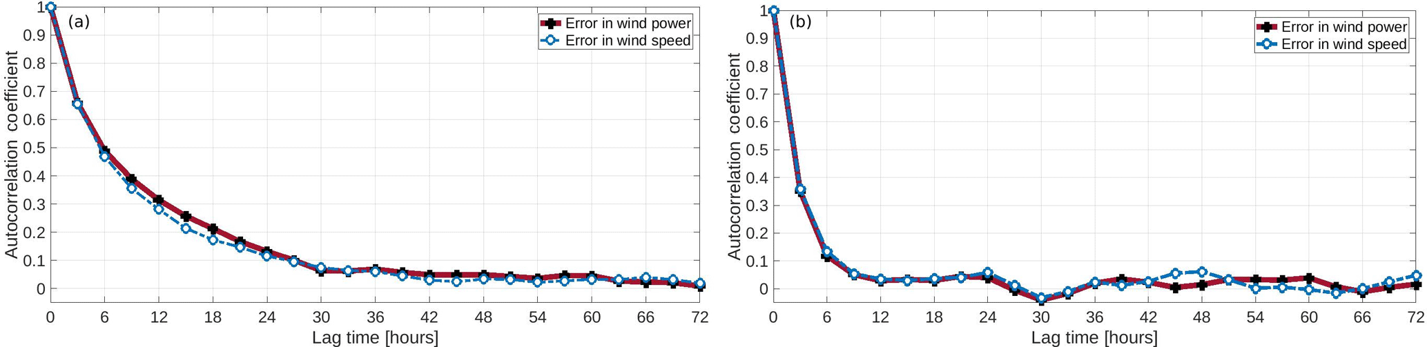
Figure 2Autocorrelation of wind speed and wind power error in time for (a) park A and (b) park C.
For the generation of the wind power probabilistic forecasts, the error distribution curve of the deterministic forecast from a previous time interval is utilized. The selection of the training period used is based on a prior analysis of the error characteristics. The following paragraphs address the points and requirements taken into consideration for the development of the methodology applied.
The temporal dependency of the forecasting error (ei), which results from the model values minus the observed ones at the same time, can be retrieved by the autocorrelation (Rc) which represents the level of similarity between a time series and its lagged version over successive time intervals, given as
In two different locations, the autocorrelation of errors both in wind speed and wind power presents a poor correlation between a current error and its past values in long time horizons (Fig. 2). In the first examined case, the errors in wind speed and wind power present some consistency for the first nine hours and are gradually reduced, tending to minimize at the end of a daily cycle. On the other hand, for the same period in another station, the relation has rapidly decreased within the first three to six hours. The demonstrated cases represent mainly a temporal and a small spatial dependency in the forecasting errors.
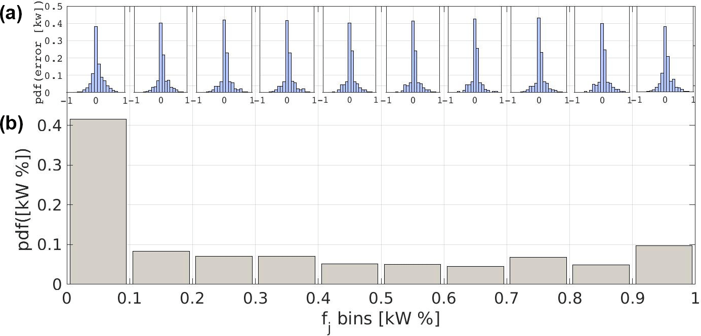
Figure 4Probability density of wind power error in the different quantiles of Pn (b) and distributions of error for each quantile (a), for park B.
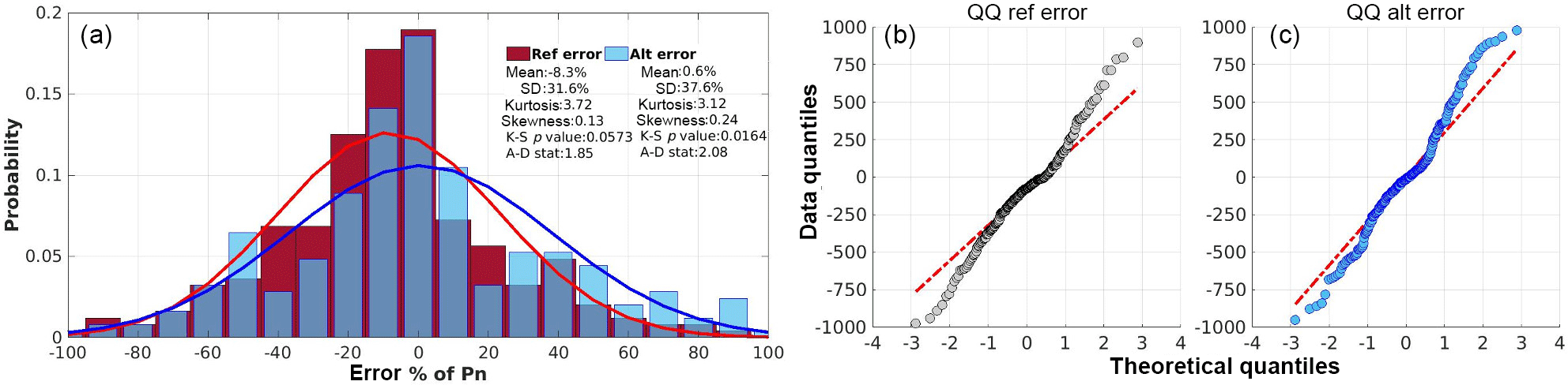
Figure 5(a) Error distributions for the Prop and Ref method, experimental and theoritical quantile-quantile error plots for (b) Ref method and (c) Prop method, in park D.
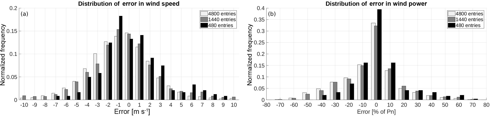
Towards the definition of the optimum selection of the previous period employed, the shaped distributions of wind speed and wind power errors of different sampling frequencies are examined. In Fig. 3 the distributions of error are presented, resulting from different sampling frequencies: 20 days (480 samples), 60 days (1440 samples) and 100 days (2400 samples). While the uncertainty in wind power forecast is related to the quality of the forecasted prevailing wind conditions, the forecasting errors of wind speed and wind power, shape different distributions. Wind speed errors are normally shaped covering a wide range of values. On the contrary, the deviations in wind power are mainly concentrated in a range between ±20 % of the nominal power (Pn), forming a more leptokurtic distribution. Moreover, it must be noted that the selection of a short historic period might exclude certain types and ranges of errors that can mislead the construction of the forecasting densities.
Additionally, the shape of deviations in different quantiles of wind power is assessed with the aim of examining the associated uncertainty under different magnitudes. Figure 4 illustrates the frequency of error occurrence in different quantiles of wind power. In addition, the distribution stemming from the errors emerging in each bin is depicted. Most of the errors occur in the ranges between 0 %–20 % and 90 %–100 % of the nominal power. This suggests an increased uncertainty in lower and maximum values of the energy yield.
The aforementioned points indicate the necessity of specific optimization techniques for the derivation of efficient probabilistic forecast methods. Error characteristics differ both spatially and temporally. A multi-period and spatially diversified training process is required, rather than one which is predetermined and uniform. Therefore, a sample of forecast errors shaping a distribution with standard deviation above the 30 % of Pn is arbitrarily considered. An analysis of twenty days is initially performed and the sample period is extended until the aforementioned criterion is met. Moreover, since the uncertainty is enhanced in certain power magnitudes, the process is recursively performed in each range of Pn, using a 10 % interval.
In order to increase the symmetry of the shaped error curve, a non-linear Kalman filtering method is utilized. Kalman filter is a dynamic approach also used in forecasting for the improvement of the initial model prediction. However, in this case the ability of extracting the random errors by the elimination of the systematic ones is further employed. Detailed descriptions and applications of the applied Kalman filtering can be found in Galanis et al. (2006). The main associated processes are stated here: The relation between the model output fi, the observed value oi and the model error ei(fi−oi) at the same time ti, can be expressed in a non-linear form as:
with ri the Gaussian non-systematic error and aj,i the coefficients that need to be defined by the process. With the elimination of the systematic error in a next forecasting interval (e.g. the next 12–48 h), the residual forecasting error is normally distributed with near zero mean value.
For the extraction of the CI, the empirical cumulative distribution of the deviation data is computed. The derived curve is approximated by a piecewise nonlinear function and the CI are further estimated. As a result, a nonparametric representation of the examined sample is obtained.
To evaluate the proposed method, termed as Prop, other methods of probabilistic forecasting are also used for comparison using the same time interval of past error values. A Reference method (Ref) is applied, calculating intervals from the model error without any other process involved. Moreover, a persistence based method (Pers) which adds and subtracts the standard deviation of observations from previous hours in each upcoming point prediction and a constant one (Const) which follows the same operation for the 20 % of nominal power, are also utilized. This value was selected in order to cover the mean absolute differences between modelled and observed power values, normalized with the nominal power of each park: 17.25 % for Park A, 14.3 % for Park B, 13 % for Park C and 18.1 % for Park D, as calculated for the whole examination period.
For the evaluation of the forecasting probabilities the reliability (PIr) and the continuous ranked probability score (CRPS) are employed. Considering an indicator Si at time ti equals to unity, if the observed value is inside the prediction bounds and zero if not, the reliability at a level of significance a is measured as the number of successful cases over the total number N of the samples:
The continuous ranked probability score combines both reliability and sharpness of the prediction intervals and is the squared difference of the modelled F(y) and the observed Fo(y) cumulative distributions:
with Fo(y) equals to unity, when the forecast variable y is above the observed value and zero otherwise. This score has a negative orientation, with smaller values suggesting better predictions.
Table 1Reliability results for the applied methods in the different parks for several confidence levels 1−a.
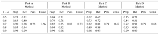
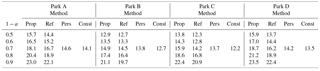
Table 2CRPS results for the applied methods in the different parks for several confidence levels 1−a.
In order to examine the implementation of the proposed methodology, a common way is to illustrate the shaped distribution and compare it against the one of the initial model error. On an indicative example, referring to Park D, the error distributions are given both for the initial model prediction (Ref method) and the prediction resulting from the application of the proposed method (Fig. 5a). The error curve produced by the Prop method presents a lower peak, with its mean centering on zero compared to the initial model prediction error. Concurrently, the standard deviation has been increased, covering a wider range of errors. Results in kurtosis and skewness parameters, which are also illustrated, demonstrate the alteration in shape that exerts with the implementation of Prop method. The lower value-closer to 3 of the kurtosis presented in Prop method indicates a higher level of normality as well as the smaller propensity of the process in producing outliers. Concerning the skewness parameter, is coequally low implying right-tailed distributions. A straightforward normality examination of the derived distributions is given by goodness of fit tests. More precisely, the Kolmogorov-Smirnov (K-S) and Anderson-Darling (A-D) are applied. In K-S test, p-values denote the threshold value of the significance level where the hypothesis for normality will be accepted compare to threshold values. In the current case, the p-value of Prop method (0.0573), suggests that the hypothesis is accepted when the critical value is close to 0.06 (i.e. for less than 94 % of the sample), while the p-value of Ref method (0.01648) suggests that the hypothesis is valid for critical value above 0.01 (99 % of the sample). On the other hand, the lower value of A-D statistics, calculated in the case of Prop method, suggests a higher goodness of fit for the normal distribution compare to the Ref method.
An additional comparison is demonstrated by the quantile-quantile (Q–Q) plots of the distributions (Fig. 5b and c). Both samples show an increased level of correlation with the normal theoretical distribution (constant line) in most ranges, while deviations appear in the lowest and highest quantiles. However, the deviations tend to be smaller in the case of Prop method as compared to the case of Ref method. It should be noted that the statistical distribution parameters used for analysing the formed distributions and quantify the level of normality, are sensitive to the size of the sample tested.
The overall performance is examined for several significance levels (a=0.1, 0.2, 0.3, 0.4, 0.5) forming intervals with confidence levels %, i.e. 50 % to 90 %. An application of the method for a specific period, with increased variability in the observed power, is illustrated in Fig. 6. The deterministic prediction follows the phase of the recorded values; however, in some cases for enclosing the recorded power, a confidence level up to 90 % is necessary.
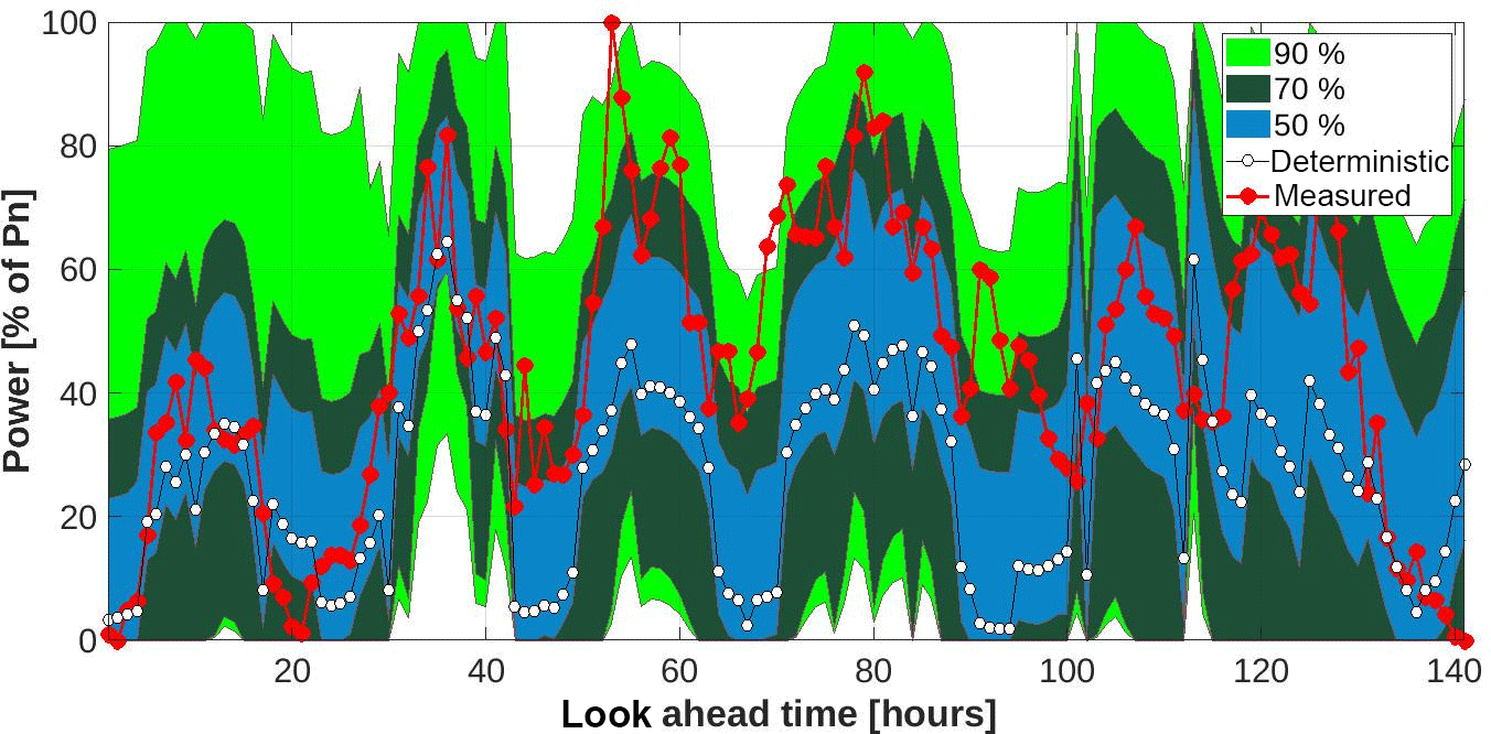
Figure 6Example of probabilistic forecast for three confidence levels % applying the Prop method, deterministic forecast and measured power time-series for park A.
Reliable and valid results are considered the ones fulfilling the baseline of %, while low CRPS values indicate prediction intervals with reliability and sharpness. Forecasting intervals stemming from the Prop method present higher reliability as compared with the ones from the Ref method (Table 1). The increment in PIr is accompanied with an increase in CRPS (Table 2). Regarding the performance of the persistence and constant method, in general both approaches present satisfactory results in relation with their simplicity; however, this is linked with the initial performance of model's prediction.
To better interpret and inter-compare the results, a threshold for defining the quality of the constructed prediction intervals is set below the 20 % of the Pn, i.e. % and % of the nominal power. Under this criterion, prediction intervals formed with significant level of 0.3 and 0.4 for Parks A and D, 0.2 and 0.3 for Park B and 0.3 for Park C for both methods tend to be more skillful. Persistence and constant methods overall fail to achieve this threshold, apart from the case-study of Park B, during the application of the persistence based method. In these cases, the reliability scores are up to 3 % higher with the application of the Prop method against the Ref method.
Deterministic wind power predictions are always susceptible to various sources of error. The construction of forecasting intervals with associated confidence levels allows the quantification of the inherent uncertainty and the provision of qualitative information on the proper utilization and decision-making issues of the generated energy yield. In this framework, a probabilistic forecasting method was proposed.
To develop the methodology, a prior analysis of the deterministic forecast error was performed. Wind speed and wind power forecasts presented different error distribution curves and a temporal dependency in the forecasting errors. Moreover, the wind power error distributions for different sampling frequencies indicated that the selection of a short historic interval as a training period might exclude certain types and ranges of errors. The analysis also implied that wind power errors can occur more frequently in certain quantiles of the nominal wind power. To address these points, a multi-period and spatially diversified training process was considered, recursively performed in each range of nominal power. A non-linear Kalman filtering algorithm was applied in different quantiles of power curve in order to eliminate the systematic part of the error and increase the symmetry of the shaped error curve. Additionally, the extraction of the confidence interval was obtained with a nonparametric approach.
The proposed methodology demonstrated the ability to improve some features related to the estimation of confidence intervals from the error shaped distributions. Symmetric-normally distributed random errors were generated with densities that cover a wide range of error magnitudes. The evaluation process and the comparison with other approaches showed that reliable probabilistic information can be achieved for certain confidence levels.
Data for Crete was provided upon request by the administrator of islands network operation department of Greece (https://www.deddie.gr/, last access: 3 September 2018). Model data in site locations is available through ftp://ftp.mg.uoa.gr/pub/chrisstath/adgeo-2018-46/ (last access: 3 September 2018).
CS performed computations, analysis and wrote the manuscript. GG aided in evaluation and NSB in model simulations. GK contributed to the final reading and suggestions.
The authors declare that they have no conflict of interest.
This article is part of the special issue “European Geosciences Union General Assembly 2018, EGU Division Energy, Resources & Environment (ERE)”. It is a result of the EGU General Assembly 2018, Vienna, Austria, 8–13 April 2018.
This work was supported by the European Commission through the Integrated
Research Programme on Wind Energy (IRPWIND), Grant Agreement 609795.
Edited by: Sonja Martens
Reviewed by: two anonymous referees
Cotton, W. R., Pielke Sr., R. A., Walko, R. L., Liston, G. E., Tremback, C. J., Jiang, H., McAnelly, R. L., Harrington, J. Y., Nicholls, M. E., Carrio, G. G., and McFadden, J. P.: RAMS 2001: Current status and future directions, Meteorol. Atmos. Phys., 82, 5–29, https://doi.org/10.1007/s00703-001-0584-9, 2003.
Galanis, G., Louka, P., Katsafados, P., Pytharoulis, I., and Kallos, G.: Applications of Kalman filters based on non-linear functions to numerical weather predictions, Ann. Geophys., 24, 2451–2460, https://doi.org/10.5194/angeo-24-2451-2006, 2006.
Jung, J. and Broadwater, R. P.: Current status and future advances for wind speed and power forecasting, Renew. Sust. Energ. Rev., 31, 762–777, https://doi.org/10.1016/j.rser.2013.12.054, 2014.
Pinson, P., Nielsen, H. A., Madsen, H., and Kariniotakis, G.: Skill forecasting from ensemble predictions of wind power, Appl. Energ., 86, 1326–1334, https://doi.org/10.1016/j.apenergy.2008.10.009, 2009.
Solomos, S., Kallos, G., Kushta, J., Astitha, M., Tremback, C., Nenes, A., and Levin, Z.: An integrated modeling study on the effects of mineral dust and sea salt particles on clouds and precipitation, Atmos. Chem. Phys., 11, 873–892, https://doi.org/10.5194/acp-11-873-2011, 2011.
Stathopoulos, C., Kaperoni, A., Galanis, G., and Kallos, G.: Wind power prediction based on numerical and statistical models, J. Wind Eng. Ind. Aerod., 112, 25–38, https://doi.org/10.1016/j.jweia.2012.09.004, 2013.
Tastu, J., Pinson, P., Trombe, P. J., and Madsen, H.: Probabilistic Forecasts of Wind Power Generation Accounting for Geographically Dispersed Information, IEEE T. Smart Grid, 5, 480–489, https://doi.org/10.1109/TSG.2013.2277585, 2014.