Evaluation of a unidirectional ATES for thermal energy supply of the State Hospital Graz South, Austria

Large-scale thermal use of shallow groundwater is often constrained in cities because temperature plumes can extend far beyond project boundaries and affect third-party water rights. Unidirectional Aquifer Thermal Energy Storage (UD-ATES) addresses this by reversing the conventional open-loop arrangement. The injection well is placed up-gradient and the production well down-gradient. During summer cooling, warmed return water is injected up-gradient; the resulting warm plume is carried by the natural groundwater flow to the down-gradient well and can be recovered in the following heating season. Conversely, during the heating season, cooled water is injected up-gradient; the resulting cold plume drifts down-gradient and can be recaptured for cooling in the next summer. This configuration is particularly suited to shallow, highly permeable aquifers with pronounced natural gradients, settings in which classical ATES suffers from advective losses, while also minimizing off-site thermal impacts that complicate permitting.

At the State Hospital Graz South site (Austria), we surveyed and characterized the aquifer and built a coupled groundwater-flow and heat-transport model to design a UD-ATES well pair tailored to local conditions. The optimized spacing between injection and production wells is ∼463 m, aligning transport time with the seasonal load profile with a peak thermal power of 1.25 MW (60 L s⁻¹ by a ΔT of 5 K). Resulting temperature anomalies remain largely confined to the property, with the thermal signal decaying to below 1 K within a few hundred metres downstream. Despite an unavoidable imbalance between heating and cooling demand over the year, the system recovers a substantial fraction of the injected energy and markedly reduces the thermal footprint compared with a conventional open loop scheme. The thermal recovery factor amounts to 0.38. An expansion of the plant to a total peak thermal power of >3.5 MW using three pairs of wells appears to be feasible at the location in question. These findings support UD-ATES as a practical pathway to decarbonize large, space-constrained consumers in high-flow aquifers while safeguarding neighbouring groundwater uses.

1 Introduction

The utilization of shallow geothermal energy in Austria began in the 1970s as a direct response to the oil crises, when rising heating oil prices highlighted the need for alternative, more cost-effective technologies (Sanner, 2016). Intrinsically linked to this transition was the technological development of heat pumps: initially, direct evaporation systems dominated, with heat pumps operating directly on horizontally arranged geothermal collectors without intermediate loops (Sanner, 2016; Lund, 2011). Between 2000 and 2010, the focus shifted to borehole heat exchangers and the thermal utilization of groundwater, making these systems the primary heat source for heat pump installations in Austria. However, since around 2010, air-source heat pumps have become the dominant system in the Austrian market due to simpler permitting procedures and easier installation (Verein Geothermie Österreich, 2025).

The potential for shallow geothermal energy in Austria is particularly significant due to its nationwide availability and decentralized applicability. The Geothermie Österreich association estimates that, with appropriate support measures, expansion could reach approximately 14 TWh of heat per year by 2040 – about 700 times today's utilization levels. Since geothermal heat is available nationwide and could benefit both small investors (homeowners) and large investors (operators of anergy networks), this technology holds substantial economic and ecological potential (Verein Geothermie Österreich, 2025).

However, conventional approaches to thermal groundwater use face significant constraints in urban areas. Extensive thermal impacts on aquifers and numerous potentially affected third-party rights complicate permitting processes in densely populated regions. In accordance with ÖWAV Guideline 207 (2009), the following rules apply in Austria: at the point where the thermally utilised groundwater is discharged into the subsoil, the temperature should not fall below 5 °C or exceed 20 °C; the maximum permissible warming/cooling of the groundwater used at the point of discharge must not exceed 6 K, based on the existing groundwater temperature at the plant location; a maximum temperature anomaly of ΔT=1 °C is permissible for third-party rights.

Seasonal thermal energy storage (TES) is a key technology for efficiently and sustainably providing heating and cooling energy. TES methods enable storage of heat from renewable sources – such as geothermal, solar energy, or industrial waste heat – in summer, which can then be reused in colder months. This approach can substantially reduce fossil fuel consumption and significantly lower CO₂ emissions (Sanner, 2016; Cabeza and Palomba, 2022).

In underground thermal energy storage (UTES), the underground serves as the storage medium. Depending on geological conditions, two main concepts are primarily implemented: Aquifer Thermal Energy Storage (ATES) and Borehole Thermal Energy Storage (BTES). Both approaches have proven commercially viable in several countries and significantly contribute to sustainable energy supply (Fleuchaus et al., 2018). Aside from ATES and BTES, other UTES variants exist, such as storing thermal energy in flooded mines or engineered rock caverns, sometimes termed cavern thermal energy storage (CTES) – and also large pit or tank thermal stores at the surface. These alternatives, however, are less common and are not directly related to aquifer use, so they are beyond the scope of this study.

ATES systems utilize groundwater to store thermal energy and recover it when needed. Energy injection and extraction typically occur via vertical wells functioning both as production and injection wells. Excess heat, for instance from solar thermal or waste heat, is injected during summer. With low groundwater flow velocities, the thermal anomaly spreads nearly radially around the injection well. During the subsequent heating period, the flow direction is reversed, turning the injection well into a production well, delivering the stored heat (Fleuchaus et al., 2020; Wesselink et al., 2018).

Due to comparatively low operating costs and large storage capacities, ATES has particularly high potential among UTES technologies (Pellegrini et al., 2019). Especially in urban areas with limited space for conventional heating and cooling systems, ATES offers an efficient, cost-effective, and environmentally friendly solution (Sommer et al., 2015). Since the 1970s, intensive research has been conducted into developing and optimizing geothermal energy systems (Sanner, 2016). However, several factors influence the efficiency of ATES, particularly groundwater flow velocities: high velocities can cause significant heat losses during seasonal storage, reducing system performance (Bloemendal and Olsthoorn, 2018). A well-established method to mitigate these losses involves installing two pairs of wells parallel to groundwater flow, compensating for heat transport via advection. For even higher efficiency, ATES installations can include a third well pair used alternately, maximizing recovery rates and optimizing heat utilization (Stemmle et al., 2024). Choosing optimal well spacing and adjusting pumping regimes are crucial to minimizing heat losses and improving system efficiency (Bloemendal and Olsthoorn, 2018; Stemmle et al., 2024). Recent studies underscore the importance of well placement: for example, Petrova et al. (2025) used stochastic modeling to show that improperly spaced ATES wells in an urban setting can lead to significant thermal interference and reduced performance, whereas an optimal spacing on the order of ∼130–160 m was found to maximize energy recovery while minimizing well-to-well interference (Petrova et al., 2025). These findings reinforce that as ATES deployment becomes denser (particularly in cities), developing generalizable well placement guidelines are essential for balancing individual system performance with overall subsurface usability.

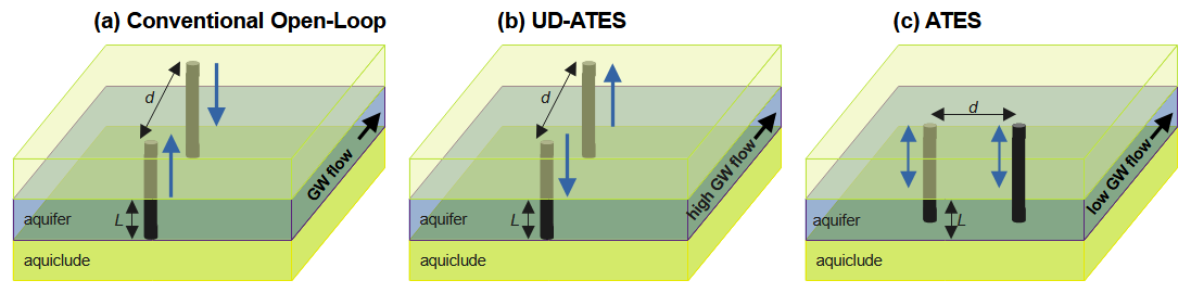
Figure 1 Schematic illustration of conventional open-loop (a), unidirectional ATES (b) and traditional ATES (c) (adapted from Silvestri et al., 2025).

Silvestri et al. (2025) introduced the concept of unidirectional ATES (UD-ATES) systems. Unlike conventional open-loop systems, where production wells are located upstream and injection wells downstream, unidirectional ATES systems reverse these roles (Fig. 1). The thermal plume injected during summer cooling reaches the production well after about six months, significantly enhancing storage efficiency. Silvestri et al. (2025) conducted numerical feasibility studies and sensitivity analyses to evaluate how well spacing, pumping schemes, and flow velocities affect recovery rates, showing maximum heat recovery rates between 55 % and 75 %. However, it should be noted that comparable or even higher recovery factors can be achieved in conventional ATES systems under conditions without significant groundwater flow. The advantages of unidirectional ATES therefore become particularly relevant in aquifers with pronounced natural groundwater movement, where advective plume drift would otherwise lead to considerable thermal losses (Ohmer et al., 2022).

A notable advantage of the unidirectional concept is the minimization of thermal anomalies in the aquifer: water cooled in winter is reused in summer, significantly reducing downstream impacts on other wells (Silvestri et al., 2025). Especially in urban areas with numerous third-party rights, such as private or drinking water wells, this can substantially improve permitting viability for larger geothermal projects.

To implement the concept described by Silvestri et al. (2025), detailed underground knowledge, a largely balanced heating-cooling ratio, and sufficient space for optimal well spacing are necessary. In the present project, the Steiermärkische Krankenanstaltengesellschaft (KAGes) plans to meet a peak load about 3.5 MW of the State Hospital Graz South's thermal power demand using shallow groundwater. In the Graz area, theuifers have excellent hydraulic properties, meaning a thermal peak load of 3.5 MW could theoretically be supplied by on the order of three well doublets with a maximum production rate of each 60 L s⁻¹.

However, a conventional open-loop design for that capacity was projected to create a thermal plume extending on the order of 3 km down-gradient – a scale that would clearly be unacceptable within the city limits of Graz (this order-of-magnitude plume length comes from preliminary site-specific modeling in this study, based on the local groundwater flow velocity and expected thermal dispersion).

This study aims to hydrogeologically test and optimize the unidirectional ATES concept for the first time in Austria. Geological maps, drilling data, and pumping test results were evaluated to create a hydrogeological conceptual model. Subsequently, a coupled flow and heat transport model was developed to determine the optimal well spacing based on local flow velocities.

Although Central Europe's climate is not entirely seasonally balanced – unlike the cosine temperature profiles typical in the Netherlands – simulation results indicate significant reductions in thermal impacts and substantial efficiency improvements in heat recovery compared to conventional open-loop systems (Silvestri et al., 2025; Jackson et al., 2024).

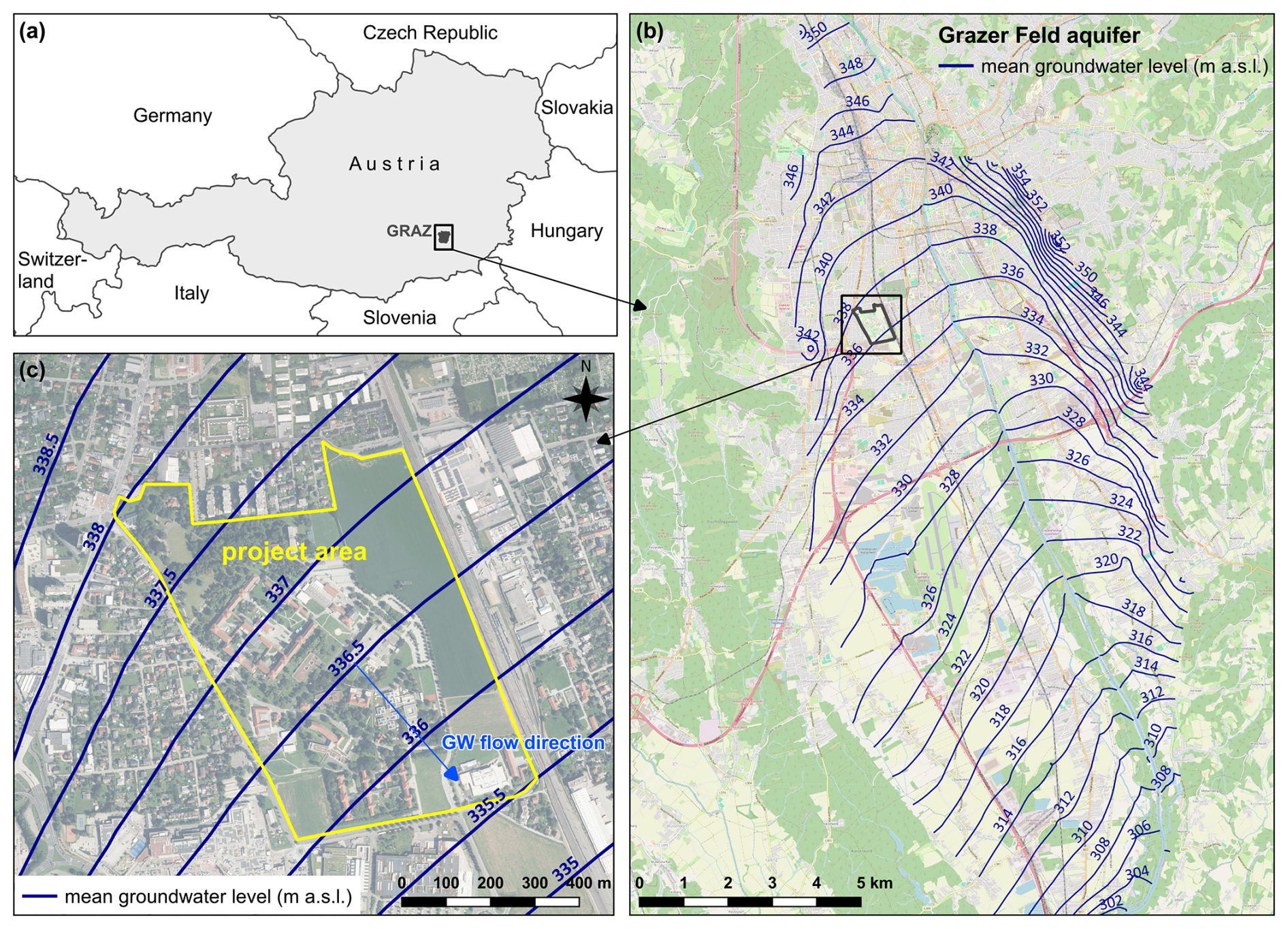
Figure 2 Overview map of the project area: location of the city of Graz within Austria (a); representation of average groundwater levels in the Graz area (b); location of the project area within the city of Graz (c) (© GIS Steiermark).

2 Study area

Graz is the second largest city in Austria and is located in the southeast of the country. The project area, which surrounds the Graz Süd Hospital, is a large site with several existing wells and is situated in the west of Graz (Fig. 2).

From a geological perspective, the project site lies on a lower terrace dating back to the Würm glacial period (Flügel and Neubauer, 1984). It consists of thick gravel layers with a low proportion of sands and fine clastic sediments. Their high hydraulic conductivity, combined with their thickness, makes them an excellent aquifer (Umweltbundesamt, 2021).

The average groundwater level in the project area ranges between 335.5 and 338.0 m above sea level, while the aquifer bottom lies between 327 and 333 m above sea level. The groundwater level has a NW-SE gradient sloping towards the receiving watercourse Mur, while the aquifer bottom has a W–E gradient (Fig. 7). This corresponds to an average groundwater thickness of approximately 5 to 9 m (Amt der Steiermärkischen Landesregierung, 2025).

The terrain elevations are between approximately 350 and 353 m above sea level, resulting in water table depths between 11 and 16 m under average groundwater conditions. An analysis of the data from the Geoportal Styria (Amt der Steiermärkischen Landesregierung, 2025) indicates a general groundwater flow direction from northwest to southeast (Fig. 2).

The basis for developing the conceptual model was provided by data on the aquifer top and characteristic groundwater levels made available through the geoportal of the Province of Styria. The large-scale distribution of the hydraulic conductivity was adopted from the regional groundwater model of the Graz Basin (Harum et al., 2007). In the area of the project site, the regional groundwater model indicates a hydraulic conductivity (k_f value) of approximately $\mathrm{3}\times {\mathrm{10}}^{-\mathrm{3}}$ to $\mathrm{5}\times {\mathrm{10}}^{-\mathrm{3}}$ m s⁻¹.

With an average groundwater gradient of I=0.0023, this results in a Darcy velocity of 6.9 to $\mathrm{11.5}\times {\mathrm{10}}^{-\mathrm{6}}$ m s⁻¹, and with an effective porosity of n_eff=0.24, a groundwater flow velocity of 2.9 to $\mathrm{4.8}\times {\mathrm{10}}^{-\mathrm{5}}$ m s⁻¹ can be calculated.

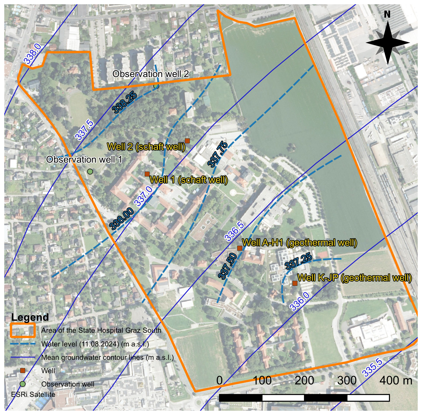
Figure 3 Groundwater contour map in the area of LKH Graz Süd on August 11, 2024 derived from new monitoring data, compared to the publicly available groundwater contour map (© GIS Steiermark).

3 Methodology

3.1 Data basis

The data basis for both the hydrogeological and the numerical model consists of publicly accessible digital data provided by the Geoportal Styria. To obtain reliable data on the local hydraulic conductivity of the aquifer, current operational data from existing wells were evaluated, and targeted pumping tests were conducted and analysed. The hydraulic tests were evaluated partly as single-well tests and partly as multi-well tests. The location of the wells is shown in Fig. 3.

To monitor changes in groundwater levels on a local scale, pressure probes with data loggers were installed in both the production wells (Well 1, Well 2, Well A-H1 and Well K-JP) and the upstream observation wells (Observation Well 1 and 2). During the pumping tests, the data recording interval was set to 1 min. Additionally, the probes recorded the groundwater temperature.

The groundwater isohypses from the project-specific measuring points, as well as those from the measurement stations of the Hydrographic Service, form the data basis for creating a groundwater contour map for the observation period. In wells with intermittent water extraction, an attempt was made to approximately extrapolate the reflected resting state of the groundwater level in order to represent the undisturbed groundwater conditions as accurately as possible in the groundwater contour map.

3.1.1 Pumping tests

One of the challenges in designing the hydraulic tests was the fact that the wells could not be taken out of service for an extended period due to the necessary water supply for the LKH facility. As a result, in some cases, operational data had to be evaluated, with the assumption of mutual influence between the wells. The hydraulic tests were carried out in two phases, in August and October 2024. In total, pumping tests were conducted and analysed at four different wells – drinking water wells 1 and 2, well A-H1 and well K-JP – located on the project site. The individual tests on the existing wells are described in the Appendix A.

The evaluation of the tests was carried out based on the hydraulic condition (steady or unsteady) and the type of well (vertical filter well or shaft well) using the following formulas:

The evaluation of the drawdown phase in a vertical filter well, assuming unsteady flow conditions in a confined aquifer, can be described by the following equation according to Theis (1935)

$$\begin{array}{}\text{(1)}& s\left(rt\right)={\displaystyle \frac{Q}{\mathrm{4}\cdot \mathit{\pi }\cdot T}}W\left(u\right)\end{array}$$

where

$$\begin{array}{}\text{(2)}& W\left(u\right)=-\mathrm{0.5772}-\ln u+u-{\displaystyle \frac{u^{\mathrm{2}}}{\mathrm{2}\cdot \mathrm{2}\mathrm{!}}}+{\displaystyle \frac{u^{\mathrm{3}}}{\mathrm{3}\cdot \mathrm{3}\mathrm{!}}}-\end{array}$$

and

$$\begin{array}{}\text{(3)}& u={\displaystyle \frac{r^{\mathrm{2}}\cdot S}{\mathrm{4}\cdot t\cdot T}}\end{array}$$

Where Q: production rate [m³ s⁻¹], W(u): Theis well function, s: drawdown [m], S: storage coefficient [–], T: transmissivity [m² s⁻¹], t: time [s], r: distance from the well or well radius [m].

The Theis well equation can also be applied in an unconfined aquifer if the drawdown s is replaced by the corrected drawdown s^′, where:

$$\begin{array}{}\text{(4)}& s^{\prime }=s-{\displaystyle \frac{s^{\mathrm{2}}}{\mathrm{2}\cdot H}}\end{array}$$

H: saturated thickness of the unconfined aquifer [m].

For small values of u (u<0.01), the drawdown in Eq. (1) can be approximated in accordance with Cooper and Jacob (1946):

$$\begin{array}{}\text{(5)}& s\left(r,t\right)={\displaystyle \frac{Q}{\mathrm{4}\cdot \mathit{\pi }\cdot T}}\left(-\mathrm{0.5772}-\ln u\right)\end{array}$$

For fully penetrating wells under unsteady flow conditions in an unconfined aquifer, the following equation (Eq. 6) from Dupuit (1863) and Thiem (1906) can be used:

$$\begin{array}{}\text{(6)}& Q=\mathit{\pi }\cdot k_{\mathrm{f}}\cdot {\displaystyle \frac{h_{\mathrm{0}}^{\mathrm{2}}-h_{\mathrm{w}}^{\mathrm{2}}}{\ln \frac{R}{r_{\mathrm{w}}}}}\end{array}$$

k_f: hydraulic conductivity [m s⁻¹]; R: radius of influence [m]; r_w: well radius [m]; h₀: static groundwater level; h_w: groundwater levels at the well [m].

For the design of shaft wells, Klimentov (1953) introduced the following equation (Eq. 7):

$$\begin{array}{}\text{(7)}& Q=\mathrm{1.366}\cdot {\displaystyle \frac{k_{\mathrm{f}}\cdot s\cdot (\mathrm{2}\cdot H_{\mathrm{a}}-s)}{\log \frac{R}{r}}}\cdot \sqrt{{\displaystyle \frac{t+\mathrm{0.5}\cdot r}{h_{\mathrm{a}}}}}\cdot \sqrt[\mathrm{4}]{{\displaystyle \frac{\mathrm{2}\cdot h_{\mathrm{a}}-t}{h_{\mathrm{a}}}}}\end{array}$$

with $R=\mathrm{3000}\cdot s\cdot \surd k_{\mathrm{f}}$ according to Sichardt, for radius of influence.

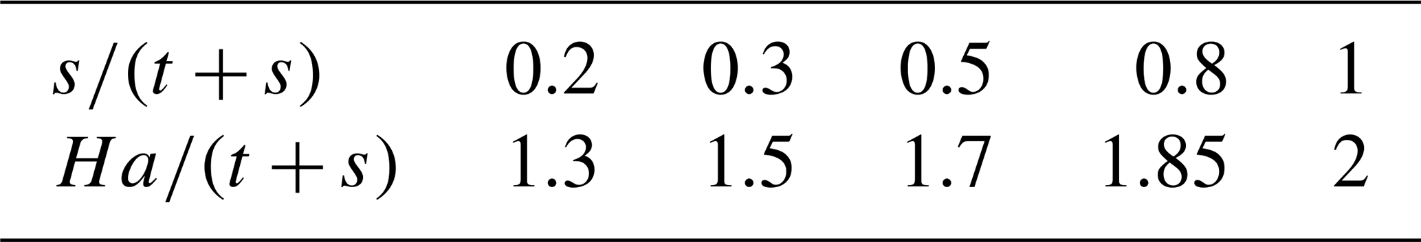
Where Q: production rate [m³ s⁻¹]; k_f: hydraulic conductivity [m s⁻¹], s: drawdown in the well [m], H_a: active inflow zone below static groundwater level [m], h_a: H_a−s distance between lowered groundwater level and the bottom of the active zone [m], t: distance between lowered groundwater level and the bottom of the well [m], H: saturated thickness (distance between static groundwater level and aquitard) [m], R: radius of influence [m], r: well radius [m].

The use of Eq. (7) assumes that part of the inflow to the well occurs through the permeable wall of the shaft. It is also assumed that the inflow to the well originates from a defined active zone below the bottom of the well, which does not necessarily correspond to the entire thickness between the well bottom and the top of the aquitard. The calculation presumes steady-state flow conditions to the well. The active zone H_a is determined according to Zamarin (1928), using the values in Table 1.

Table 1 Reference table for identifying the active inflow zone.

3.1.2 Assessment of thermal efficiency

One of the main indicators of thermal performance is the heat recovery ratio or thermal recovery efficiency. It represents the ratio of recovered thermal energy to the total thermal energy initially transferred and stored in the shallow geothermal reservoir (Gil et al., 2022; Sommer at al., 2015).

$$\begin{array}{}\text{(8)}& {\mathit{\eta }}_{\mathrm{th}}={\displaystyle \frac{E_{\mathrm{recovered}}}{E_{\mathrm{stored}}}}\end{array}$$

Where the energy recovered E_recovered is calculated as the sum of the abstracted water flow rates Q considering the temperature difference between the abstracted groundwater T₀ and the reinjection temperature of the aquifer T_B, the volumetric heat capacity of the groundwater C_w produced for extraction time.

$$\begin{array}{}\text{(9)}& E_{\mathrm{recovered}}=\underset{\mathrm{0}}{\overset{t}{\int }}Q\cdot \left(T_{\mathrm{0}}-T_{\mathrm{B}}\right)\cdot C_{\mathrm{w}}\mathrm{d}t\end{array}$$

The stored energy E_stored is calculated as the sum of the injected water flow rates Q considering the temperature difference between the injected water T_in and the background temperature of the aquifer T_B, the volumetric heat capacity of the water C_w injected at an injection time.

$$\begin{array}{}\text{(10)}& E_{\mathrm{stored}}=\underset{\mathrm{0}}{\overset{t}{\int }}Q\cdot \left(T_{\mathrm{in}}-T_{\mathrm{B}}\right)\cdot C_{\mathrm{w}}\mathrm{d}t\end{array}$$

3.2 Analytical models

Analytical models are based on analytical solutions to the initial and boundary-value problems that result from the physical processes considered and their governing differential equations (Kinzelbach, 1987). They make it possible to estimate hydraulic and thermal processes in an idealised, isotropic aquifer using few input parameters and with low computational effort. Processes such as interactions between installations and receiving waters, changes in flow velocity and direction, convective heat gains/losses, or operational transients cannot be represented within this idealised framework.

3.2.1 1D solution

The one-dimensional heat propagation in the aquifer is most easily described using an analytical solution of the advective heat conduction equation (advection without dispersion/diffusion):

$$\begin{array}{}\text{(11)}& {\displaystyle \frac{\partial T}{\partial t}}+v_{\mathrm{a}}{\displaystyle \frac{\partial T}{\partial x}}=\mathrm{0}\text{(12)}& {\displaystyle }T(x,t)=T_{\mathrm{0}}\cdot \left(x-v_{\mathrm{a}}\cdot t\right)\end{array}$$

The one-dimensional heat propagation in an aquifer can be described more accurately using the advection-dispersion heat equation, taking heat storage into account. For design purposes an analytical step input is used.

$$\begin{array}{}\text{(13)}& R_{\mathrm{th}}{\displaystyle \frac{\partial T}{\partial t}}+v_{\mathrm{a}}{\displaystyle \frac{\partial T}{\partial x}}={\displaystyle \frac{\partial }{\partial x}}\left(D_{\mathrm{L}}{\displaystyle \frac{\partial T}{\partial x}}\right)\end{array}$$

For a point input the solution takes a Gaussian form (in the longitudinal direction).

$$\begin{array}{}\text{(14)}& \mathrm{\Delta }T(x,t)={\displaystyle \frac{\mathrm{\Delta }{T}_{\mathrm{inj}}\cdot c_{\mathrm{w}}\cdot Q}{\sqrt{(\mathrm{4}\mathit{\pi }\cdot {\mathit{\alpha }}_{\mathrm{L}}\cdot t)}}}\cdot \exp \left(-{\displaystyle \frac{{\left(x-v_{\mathrm{a}}\cdot t\right)}^{\mathrm{2}}}{\mathrm{4}\cdot {\mathit{\alpha }}_{\mathrm{L}}\cdot t}}\right)\end{array}$$

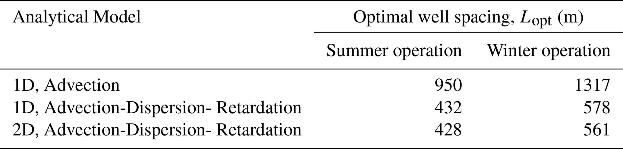
The optimal well spacing is computed from the following expression:

$$\begin{array}{}\text{(15)}& L\left(t,r\right)={\displaystyle \frac{v_{\mathrm{a}}}{R}}\cdot t+\mathrm{2}\sqrt{{\displaystyle \frac{D_{\mathrm{L}}}{R}}\cdot t}\cdot {\text{erfc}}^{-\mathrm{1}}\left(\mathrm{2}r\right)\end{array}$$

with

$$\begin{array}{}\text{(16)}& D_{\mathrm{L}}={\displaystyle \frac{{\mathit{\lambda }}_{\mathrm{m}}}{n_{\mathrm{e}}{c}_{\mathrm{w}}}}+{\mathit{\alpha }}_{\mathrm{L}}\cdot v_{\mathrm{a}}\end{array}$$

and

$$\begin{array}{}\text{(17)}& R_{\mathrm{th}}={\displaystyle \frac{\left(\mathrm{1}-n_{\mathrm{e}}\right)\cdot c_{\mathrm{s}}+n_{\mathrm{e}}\cdot c_{\mathrm{w}}}{n_{\mathrm{e}}\cdot c_{\mathrm{w}}}}\end{array}$$

as well as

$$\begin{array}{}\text{(18)}& r={\displaystyle \frac{\mathrm{\Delta }T(L,t)}{\mathrm{\Delta }{T}_{\mathrm{inj}}}}=\mathrm{0.1}\end{array}$$

3.2.2 2D Solution

For horizontal flow in the x direction (y transverse to flow) the temperature field is governed by the retarded ADE in a saturated porous medium without vertical heat losses:

$$\begin{array}{}\text{(19)}& R_{\mathrm{th}}{\displaystyle \frac{\partial T}{\partial t}}+v_{\mathrm{a}}{\displaystyle \frac{\partial T}{\partial x}}={\displaystyle \frac{\partial }{\partial x}}\left(D_{\mathrm{L}}{\displaystyle \frac{\partial T}{\partial x}}\right)+{\displaystyle \frac{\partial }{\partial y}}\left(D_T{\displaystyle \frac{\partial T}{\partial y}}\right)\end{array}$$

with

$$\begin{array}{}\text{(20)}& \begin{array}{rl}{R}_{\mathrm{th}}& =\mathrm{1}+{\displaystyle \frac{{\mathit{\rho }}_{\mathrm{b}}\cdot c_{\mathrm{s}}}{n_{\mathrm{eff}}\cdot {\mathit{\rho }}_{\mathrm{W}}\cdot c_{\mathrm{W}}}}\\ & ={\displaystyle \frac{n_{\mathrm{eff}}\cdot {\mathit{\rho }}_{\mathrm{W}}\cdot c_{\mathrm{W}}+(\mathrm{1}-n_{\mathrm{eff}})\cdot {\mathit{\rho }}_{\mathrm{G}}\cdot c_{\mathrm{G}}}{n_{\mathrm{eff}}\cdot {\mathit{\rho }}_{\mathrm{W}}\cdot c_{\mathrm{W}}}}\end{array}\end{array}$$

and

$$\begin{array}{}\text{(21)}& R_{\mathrm{th}}{\displaystyle \frac{\partial T}{\partial t}}+v_{\mathrm{a}}{\displaystyle \frac{\partial T}{\partial x}}={\displaystyle \frac{\partial }{\partial x}}\left(D_{\mathrm{L}}{\displaystyle \frac{\partial T}{\partial x}}\right)+{\displaystyle \frac{\partial }{\partial y}}\left(D_{\mathrm{T}}{\displaystyle \frac{\partial T}{\partial y}}\right)\end{array}$$

and

$$\begin{array}{}\text{(22)}& D_{\mathrm{L}}={\mathit{\alpha }}_{\mathrm{L}}{v}_{\mathrm{a}}+{\mathit{\kappa }}_{\mathrm{eff}}\text{ and }{D}_{\mathrm{T}}={\mathit{\alpha }}_{\mathrm{T}}{v}_{\mathrm{a}}+{\mathit{\kappa }}_{\mathrm{eff}}\end{array}$$

This describes the temperature field of a continuous step input of heat in a homogeneous, confined aquifer under transient conditions. In the planar model the source is represented as a vertical plane (capture width) perpendicular to flow.

$$\begin{array}{}\text{(23)}& \begin{array}{rl}\mathrm{\Delta }T(x,y,t)& ={\displaystyle \frac{Q\cdot \mathrm{\Delta }{T}_{\mathrm{inj}}}{\mathrm{4}\cdot n_{\mathrm{e}}\cdot m\cdot v_{\mathrm{a}}\cdot \sqrt{(\mathit{\pi }\cdot {\mathit{\alpha }}_T)}}}\cdot \exp \left({\displaystyle \frac{x-r}{\mathrm{2}\cdot {\mathit{\alpha }}_{\mathrm{L}}}}\right)\\ & \cdot {\displaystyle \frac{\mathrm{1}}{\sqrt{r}}}\cdot \text{erfc}\left({\displaystyle \frac{r-v_{\mathrm{a}}\cdot t/R}{\mathrm{2}\cdot \sqrt{v_{\mathrm{a}}\cdot {\mathit{\alpha }}_{\mathrm{L}}\cdot t/R}}}\right)\end{array}\end{array}$$

with

$$\begin{array}{}\text{(24)}& r=\sqrt{x^{\mathrm{2}}+y^{\mathrm{2}}{\displaystyle \frac{{\mathit{\alpha }}_{\mathrm{T}}}{{\mathit{\alpha }}_{\mathrm{T}}}}}\end{array}$$

Where: ΔT: target isotherm (difference from the undisturbed groundwater temperature) [°C]; ΔT_inj: injection temperature difference (relative to the undisturbed groundwater temperature) [°C]; v_a: pore (seepage) velocity [m s⁻¹; R_th: thermal retardation factor [–]; D_L, D_T: longitudinal and transverse thermal dispersion coefficients (m² s⁻¹); α_L, α_T: longitudinal and transverse dispersivities (m); λ_m: effective thermal conductivity of the porous medium [W m⁻¹ K⁻¹)]; n_e: effective porosity [–]; c_w, c_s: volumetric heat capacities of water and solid matrix [J m⁻³ K⁻¹)].

Using the capture width:

$$\begin{array}{}\text{(25)}& W_{\mathrm{c}}={\displaystyle \frac{Q}{m\cdot n_{\mathrm{e}}\cdot v_{\mathrm{a}}}}\end{array}$$

For unidirectional ATES design the temperature peak (centroid) should reach the abstraction well only after the storage time t_s. Without an explicit safety factor the optimal spacing from peak matching is:

$$\begin{array}{}\text{(26)}& L_{\mathrm{0}}={\displaystyle \frac{v_{\mathrm{a}}}{R_{\mathrm{th}}}}{t}_{\mathrm{s}}\end{array}$$

Because the plume broadens due to dispersion, an empirical, reliability-based margin is added along the flow direction (e.g. γ=1.96 for ≈95 % coverage):

$$\begin{array}{}\text{(27)}& L_{\mathrm{opt}}={\displaystyle \frac{v_{\mathrm{a}}}{R_{\mathrm{th}}}}{t}_{\mathrm{s}}+\mathit{\gamma }\sqrt{{\displaystyle \frac{\mathrm{2}\cdot D_{\mathrm{L}}}{R_{\mathrm{th}}}}}{t}_{\mathrm{s}}\end{array}$$

The calculation bases for the analytical models are summarised in Table 2.

Table 2 Physical properties of the aquifer (Österreichische Wasser- und Abfallwirtschaftsverband, 2009; VDI, 2010; Lemmon et al., 2025).

Properties of water at 13 °C.

3.3 Numerical model

To account for all physical properties governing heat transport in groundwater – such as conduction, advection, and hydrodynamic dispersion – the groundwater simulation software FEFLOW (Diersch, 2014) was used. This numerical 3D finite element model (FEM) solves the coupled differential equations of groundwater flow and heat transport, enabling the simulation of groundwater extraction and reinjection from wells, as well as the hydrodynamic regime and thermal transport.

Based on the collected data, a numerical model of groundwater flow and heat transport was developed. A simplified two-dimensional, horizontal, unsteady groundwater model was created. The model extent was chosen so that the thermal effects of the simulations for optimizing the planned pilot plant could be captured until they dissipated. The relatively small model area of 2.22 km² was made possible by the unconventional, reversed arrangement of the wells, designed as a unidirectional ATES system.

The model domain was defined between the groundwater contour lines 338.0 m a.s.l. (inflow boundary in the northwest) and 334.0 m a.s.l. (outflow boundary in the southeast), which served as hydraulic boundary conditions within the model. At the northwest inflow boundary, the thermal boundary condition was defined by an assumed constant temperature of T=13 °C. No other groundwater extractions were considered within the model domain. The extraction and reinjection rates as well as the corresponding temperature differences can be found in Table 3.

Table 3 Extraction and reinjection rates and temperature differential – for the “West” well pair.

4 Results

4.1 Groundwater level and temperature measurements

The groundwater isohypses from project-specific monitoring points, along with data from Hydrographic Service stations, serve as the basis for generating a groundwater contour map for the observation period. In wells subject to intermittent water extraction, extrapolation was applied to estimate the static groundwater level, aiming to represent the undisturbed resting state of groundwater as accurately as possible in the contour map (see Fig. 3).

4.2 Pump Test Evaluations

4.2.1 Wells 1 and 2

Wells 1 and 2 are large-diameter shaft wells: Well 1 has a shaft bottom diameter of D=5 m, while Well 2 has a shaft diameter of D=3 m. The pumping durations were relatively short compared to the storage volumes of the shafts.

An evaluation of the pumping test data using the Dupuit-Thiem method is not feasible, as the wells in question are imperfect, large-diameter shaft wells whose inflow behavior deviates significantly from the assumptions underlying the Dupuit model. The same applies to unsteady-state evaluations based on the Theis well equation (Kruseman and de Ridder, 1994).

Therefore, the semi-empirical formula developed by Klimentov (1953) for shaft wells was used in order to at least obtain indicative values for local hydraulic conductivity around the wells.

In Well 1, three test phases were evaluated. With nearly constant pumping rates of approximately Q=12.7 L s⁻¹, quasi-steady drawdowns of about s=0.25 m were generated (see Fig. A1).

Using the values H=6.5 m, H_a=2.51 m, t=2.3 m, and r=2.5 m, a hydraulic conductivity of $k_{\mathrm{f}}=\mathrm{9.1}\times {\mathrm{10}}^{-\mathrm{3}}$ m s⁻¹ was determined.

In addition, the response in Well 1 to the test phase conducted in Well 2 (Fig. A2) was evaluated (Fig. 4). No disturbances from other water withdrawals were observed in either well during the test. The evaluation yielded a transmissivity of $T=\mathrm{1.19}\times {\mathrm{10}}^{-\mathrm{1}}$ m² s⁻¹ and, assuming an average saturated thickness of H=6.5 m between Wells 1 and 2, a hydraulic conductivity of $k_{\mathrm{f}}=\mathrm{1.83}\times {\mathrm{10}}^{-\mathrm{2}}$ m s⁻¹.

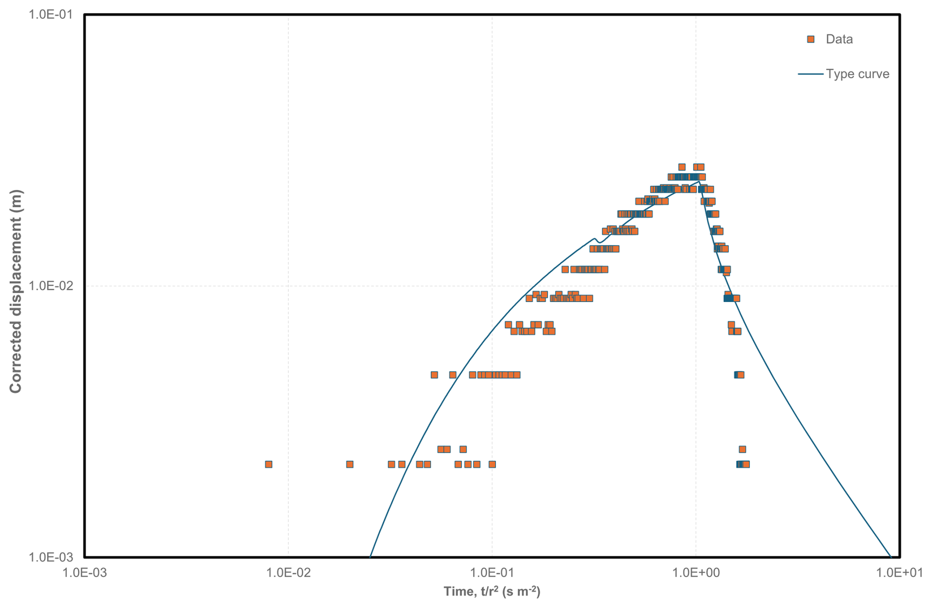
Figure 4 Evaluation of the response in Well 1 to the pumping phase in Well 2 on 20 October 2024, based on Theis (drawdown and recovery phase).

4.2.2 Well A-H1 Geothermal

For Well A-H1 Geothermal, an approximately 7 h unsteady drawdown phase on 20 August 2024, was selected for evaluation (Fig. A4). The analysis yielded a transmissivity of $T=\mathrm{1.0}\times {\mathrm{10}}^{-\mathrm{1}}$ m² s⁻¹, and with a saturated thickness of H=9.94 m, a hydraulic conductivity of $k_{\mathrm{f}}=\mathrm{1.0}\times {\mathrm{10}}^{-\mathrm{2}}$ m s⁻¹ was determined (Fig. 5).

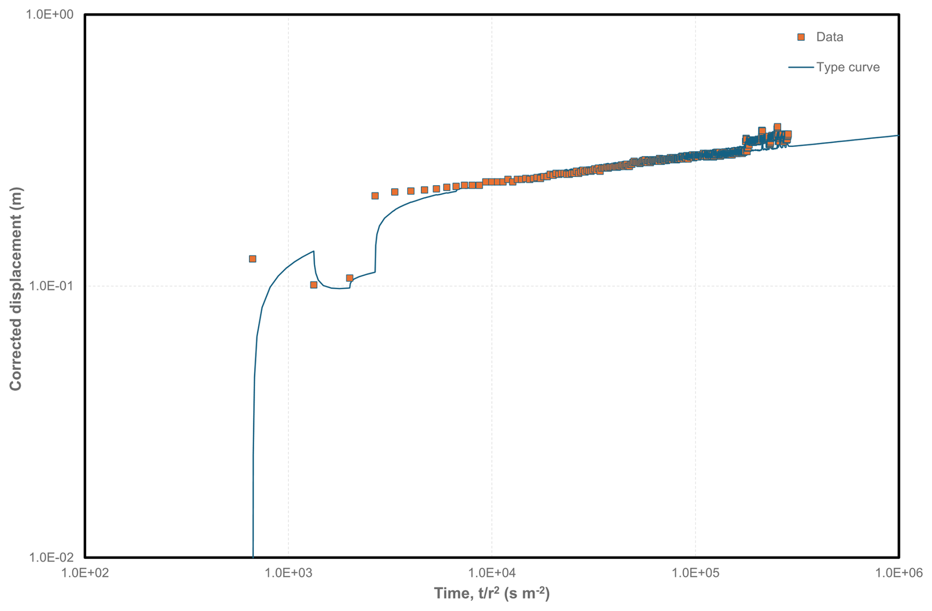
Figure 5 Evaluation of the pumping phase on 20 August 2024, in Well A-H1 Geothermal according to Theis.

4.2.3 Well K-JP Geothermal

In Well K-JP Geothermal, an approximately 12 h unsteady drawdown phase on 9 August 2024, was selected for evaluation (Fig. A6). The analysis yielded a transmissivity of $T=\mathrm{4.85}\times {\mathrm{10}}^{-\mathrm{2}}$ m² s⁻¹, and with a saturated thickness of H=8.18 m, a hydraulic conductivity of $k_{\mathrm{f}}=\mathrm{5.09}\times {\mathrm{10}}^{-\mathrm{3}}$ m s⁻¹ was determined (Fig. 6). Table 4 summarizes the hydraulic conductivities determined from the pumping tests.

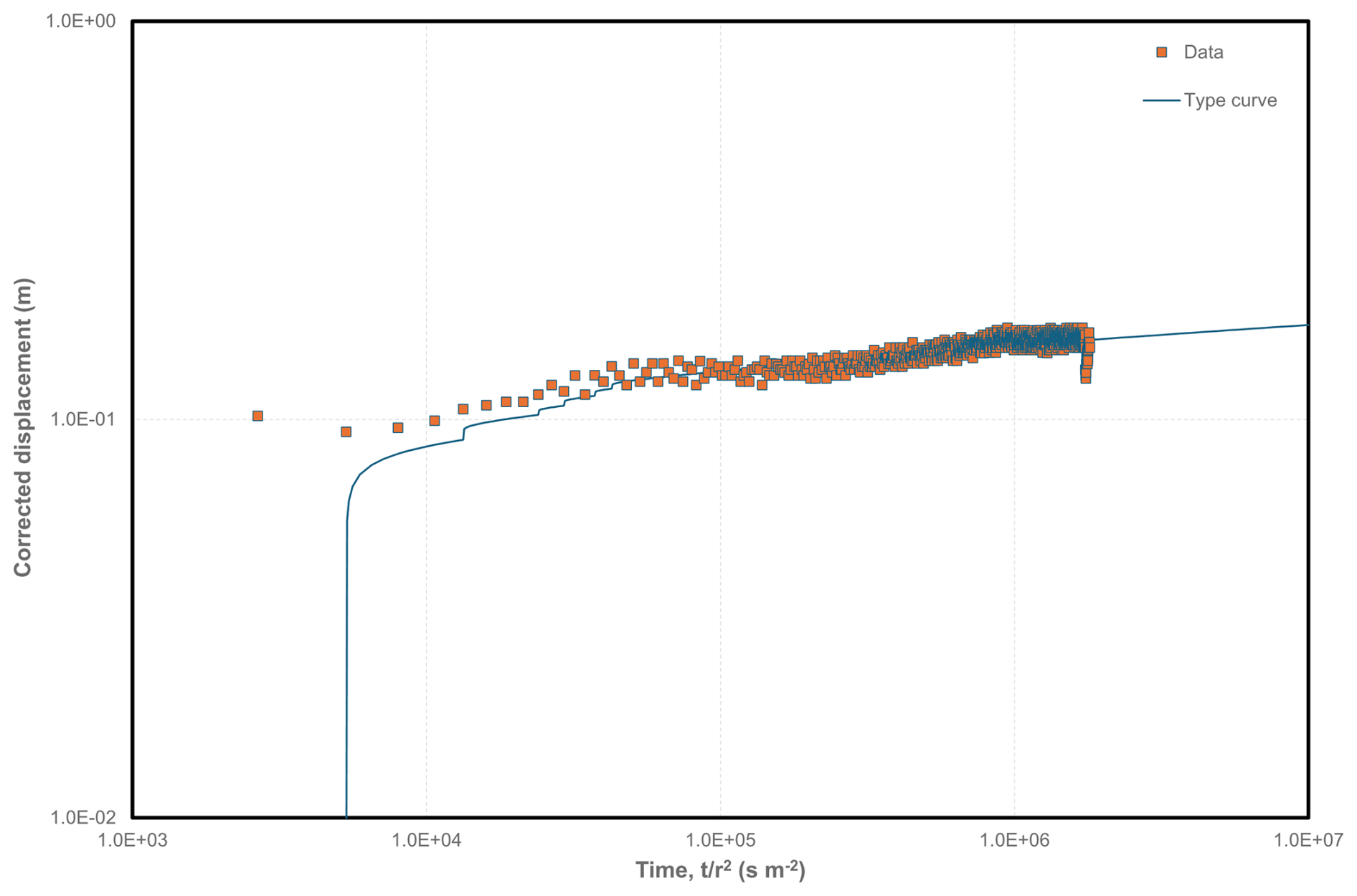
Figure 6 Evaluation of the pumping phase on 9 August 2024, in Well K-JP Geothermal according to Theis.

Table 4 Summary of the determined hydraulic conductivities.

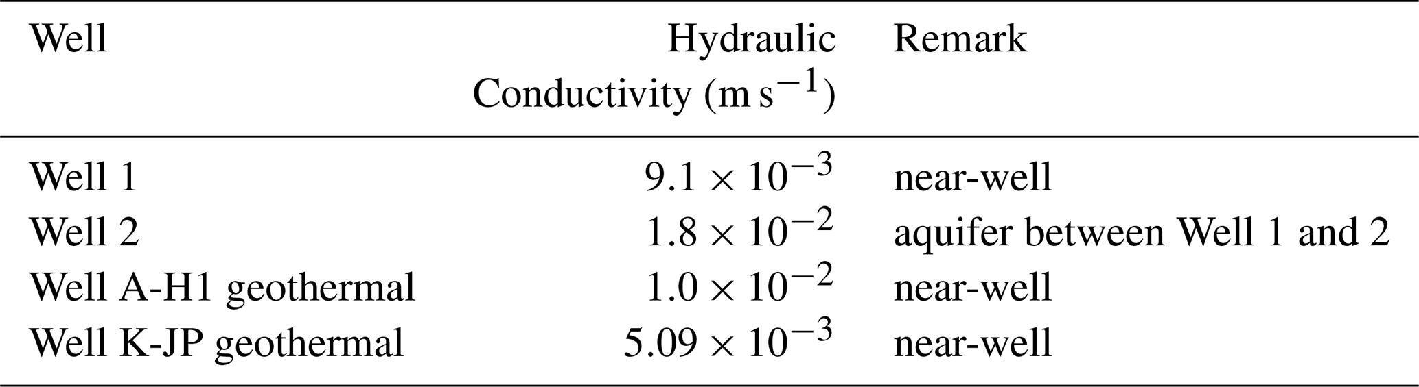
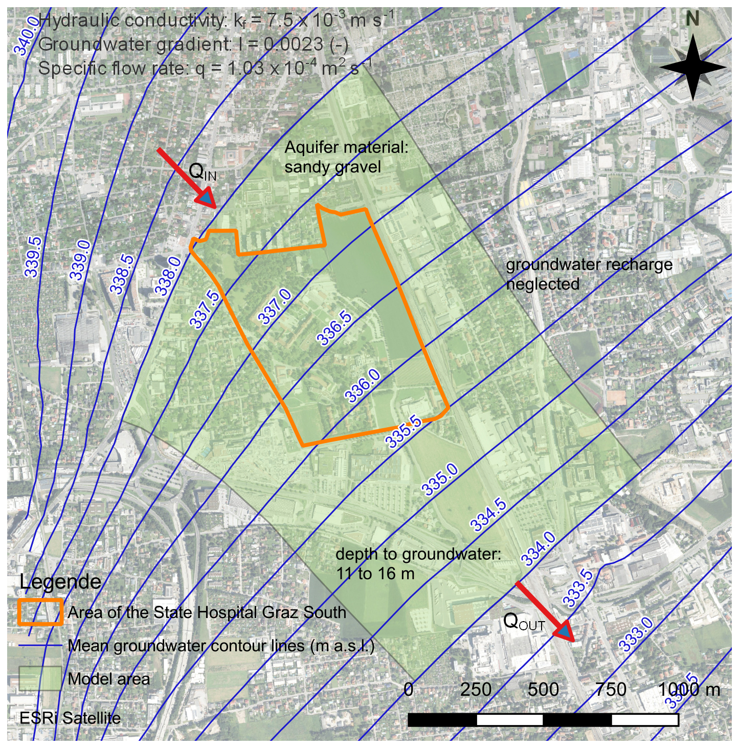
Figure 7 Sketch of the hydrogeological model (© GIS Steiermark).

4.3 Hydrogeological conceptual model

The elements of the hydrogeological model are schematically summarized in Fig. 7. The aquifer, composed of sandy gravel, has a saturated thickness of H=5 to 9 m. The depth to groundwater varies between 11 and 16 m. The general flow direction is from NW to SE, with an average hydraulic gradient of I=0.0023 (see Fig. 7). Based on locally determined values, a hydraulic conductivity of $k_{\mathrm{f}}=\mathrm{7.5}\times {\mathrm{10}}^{-\mathrm{3}}$ m s⁻¹ is assumed uniformly across the model area. This results in a specific discharge of q=7.45 to 13.41 m³ d⁻¹ m⁻¹. Groundwater recharge is neglected in the model.

For simplicity, the dispersivity was estimated based on the assumption – following de Marsily (1986) – that the dispersivities for solute transport and heat transport are identical, and thus the relationships established for solute transport were applied.

Xu and Eckstein (1995) published a formula for estimating the longitudinal dispersivity (in meters) as a function of the length of the contaminant plume (liters in meters):

$$\begin{array}{}\text{(28)}& {\mathit{\alpha }}_{\mathrm{L}}=\mathrm{0.83}\cdot ({\log }_{\mathrm{10}}L{)}^{\mathrm{2.414}}\end{array}$$

With the projected length of the thermal plume preliminarily estimated at 400 to 500 m, based on the specific arrangement of extraction and injection wells, a longitudinal dispersivity of α_L=8 m was assumed for the simulations, along with a ratio of ${\mathit{\alpha }}_{\mathrm{L}}/{\mathit{\alpha }}_{\mathrm{T}}=\mathrm{10}$ (Bundschuch and Suares Arrige, 2010).

The hydraulic and thermal parameters of the aquifer and other simulation fundamentals are shown in Table 5.

Table 5 Summary of the results of the analytical models.

4.4 Analytical Models – Results

The optimal well spacing calculated using the analytical models described in Sect. 3.2 based on the hydraulic and thermal parameters summarised in Table 3 is shown in Table 5.

4.5 Numerical Model – Simulation Results

Optimization of the First Well Pair

In the model, the positions of the extraction and reinjection wells were each varied approximately along the streamline – constructed for the mean groundwater level (mGW) conditions – connecting the two wells. The aim of the optimization was to determine the distance between the extraction and reinjection wells such that:

1. the residual thermal plume passing the extraction well would exert minimal thermal impact downstream on existing water rights, and

2. an optimal efficiency of heat recovery could be achieved.

Since the energy input during the cooling season exceeds the energy extraction during the heating season, there is no thermal balance in the groundwater system (see Table 2). Consequently, a residual thermal plume will develop and pass the extraction well, continuing downstream.

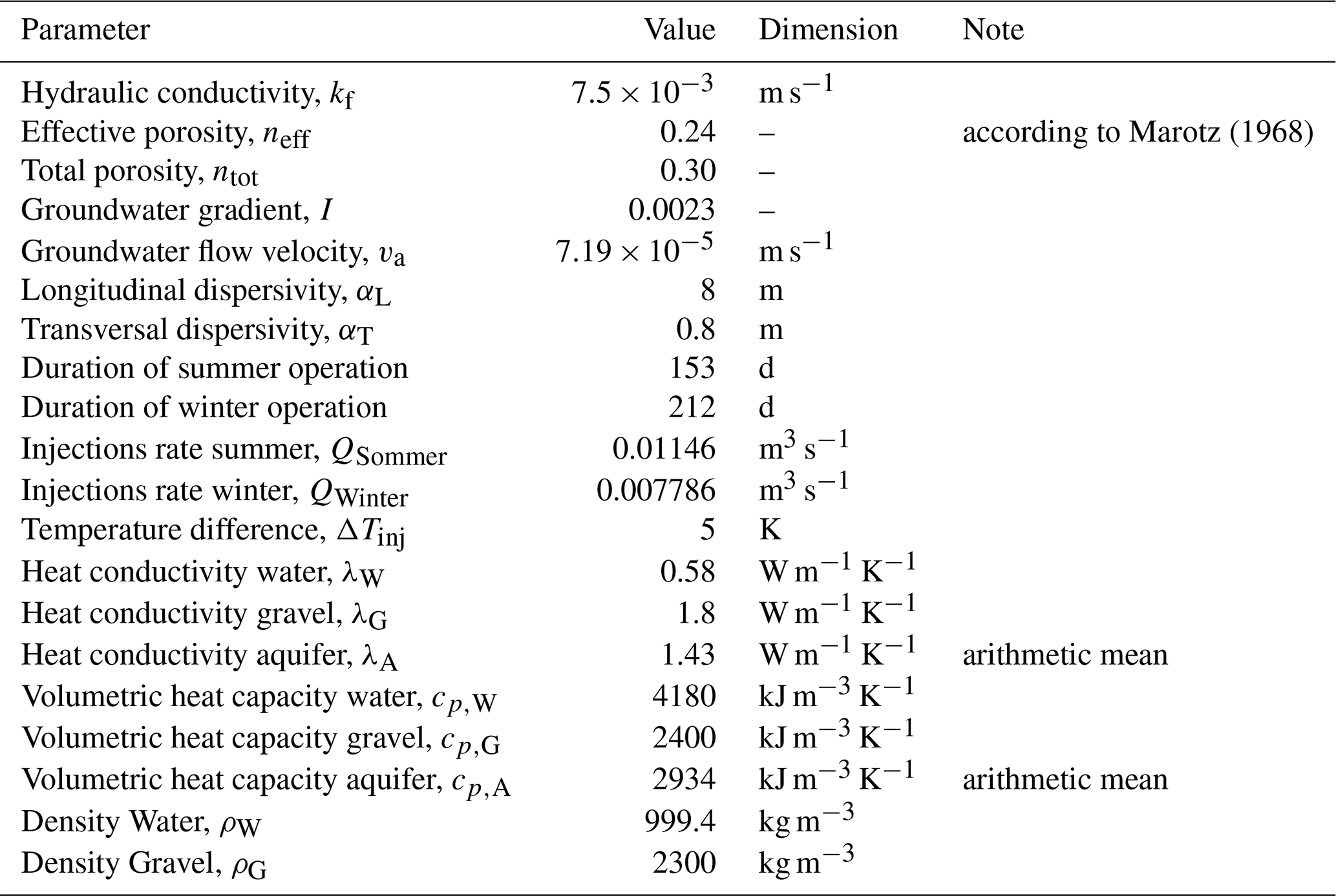
The simulations were conducted over a period of five years, each starting on 1 January. A five-year duration proved sufficient, as a periodically recurring thermal pattern in the aquifer established by that time, and the large-scale thermal effects dissipated within the model domain.

The internal hydraulic and thermal boundary conditions were defined based on the load data of the well pair – extraction and reinjection rates, and temperature differential (see Table 2). The monthly average extraction and reinjection rates correspond to peak loads of 30–35 L s⁻¹ during heating and 40–45 L s⁻¹ during cooling.

The potential locations of the extraction and reinjection wells were determined along streamlines, taking into account the two additional well pairs planned in the western part of the project area. When situating the wells, existing buildings and roads had to be considered. The reinjection wells in the north could only be placed outside the protection zones of wells 1 and 2. As a result, only a narrow area close to the western boundary of the project site was available.

In the final variant, the reinjection well was slightly shifted northwest. The location of the extraction well was determined along the corresponding streamline. After several simulation runs, the optimized distance between reinjection and extraction wells was established at approximately 463 m. The simulation results of the optimisation are summarised in Table 6.

Table 6 Simulation results for different well spacing. Bolded text: optimized spacing between injection and production wells.

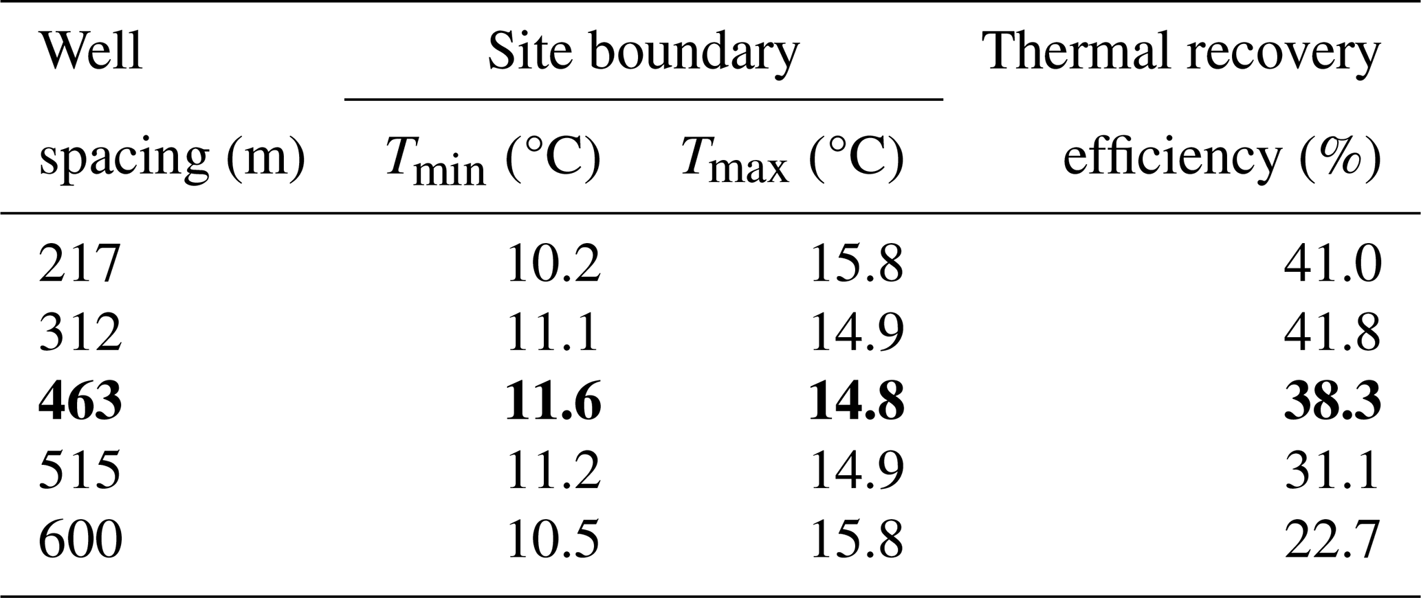
T_min and T_max represent in Table 6 the minimum and maximum temperatures at the intersection of the corresponding streamline and the property boundary. The control points along the streamline running through the extraction well and along the site boundary approximately perpendicular to the flow are shown in Fig. 8.

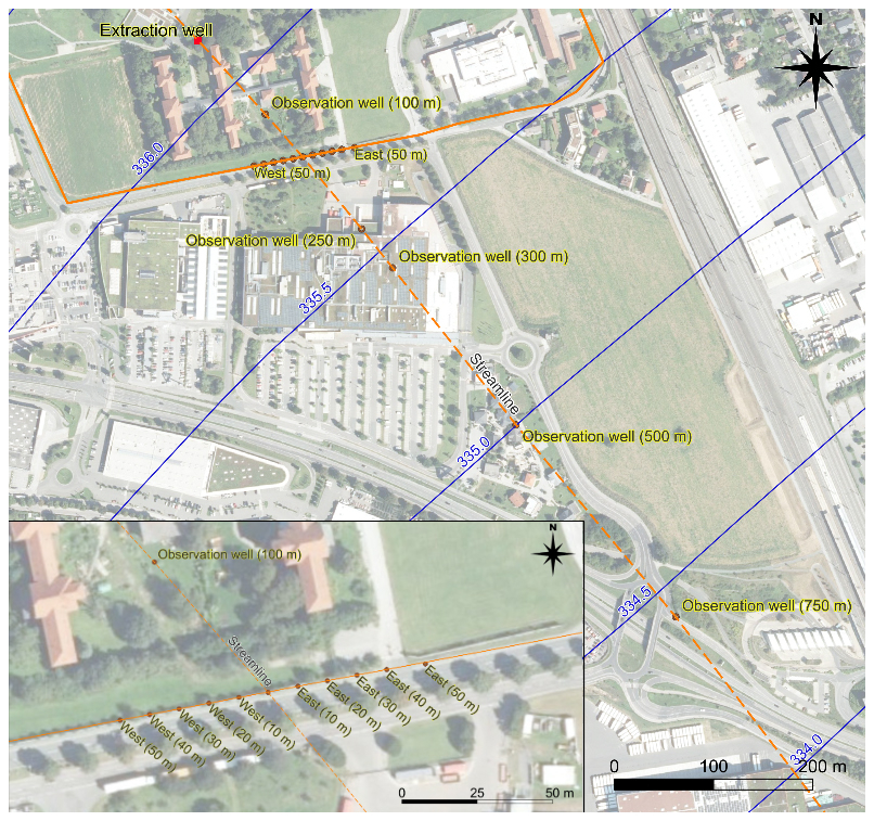
Figure 8 Location of control points along the streamline running through the extraction well and along the site boundary (© GIS Steiermark).

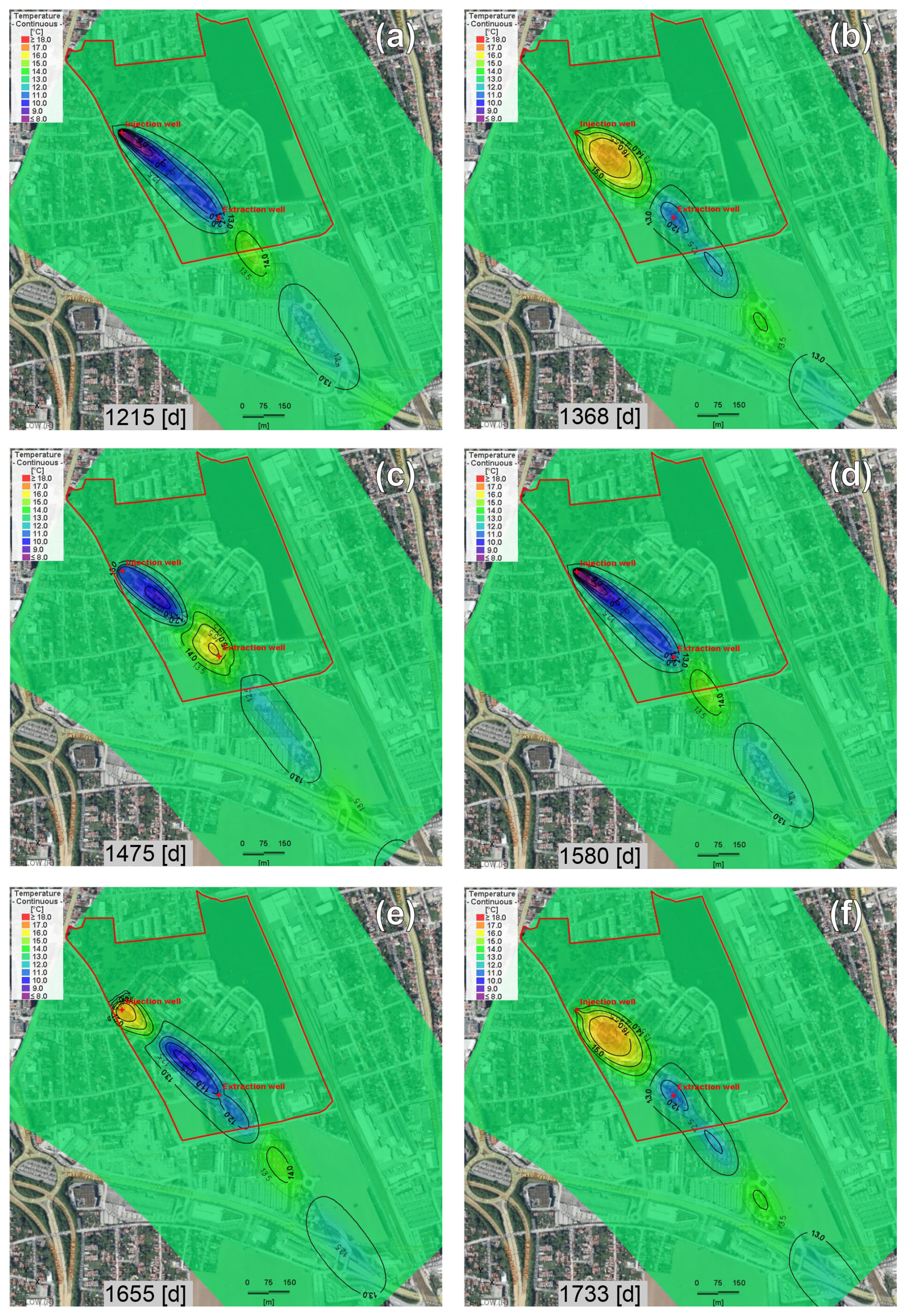
Figure 9 Illustration of the temperature distributions during and at the end of the heating and cooling periods. The states are as follows: (a) at the end of the heating period (end of April) in the 4th year of operation; (b) at the end of the heating period (end of September) in the 4th year of operation; (c) in the middle of the heating period (mid-January) in the 5th year of operation; (d) at the end of the heating period (end of April) in the 5th year of operation; (e) in the middle of the cooling period (mid-July) in the 5th year of operation; (f) at the end of the cooling period (end of September) in the 5th year of operation (© GIS Steiermark).

The variant with a well spacing of 463 m was selected for implementation in consultation with the operator. As can be seen from the spatial-temporal development of the thermal plume in Fig. 9, the cold plume (ΔT<1 °C) disappears approximately 160 m southeast of the southern property boundary, while the heat plume loses its thermal effect (ΔT<1 °C) about 405 m downstream beyond the southern boundary of the site, causing no risk to third-party water rights.

Of particular interest is the temperature at which the plume reaches the property boundary, as outside the property, third-party water rights could be thermally affected. The temperature profiles with which the plume passes the site boundary is shown in Fig. 10.

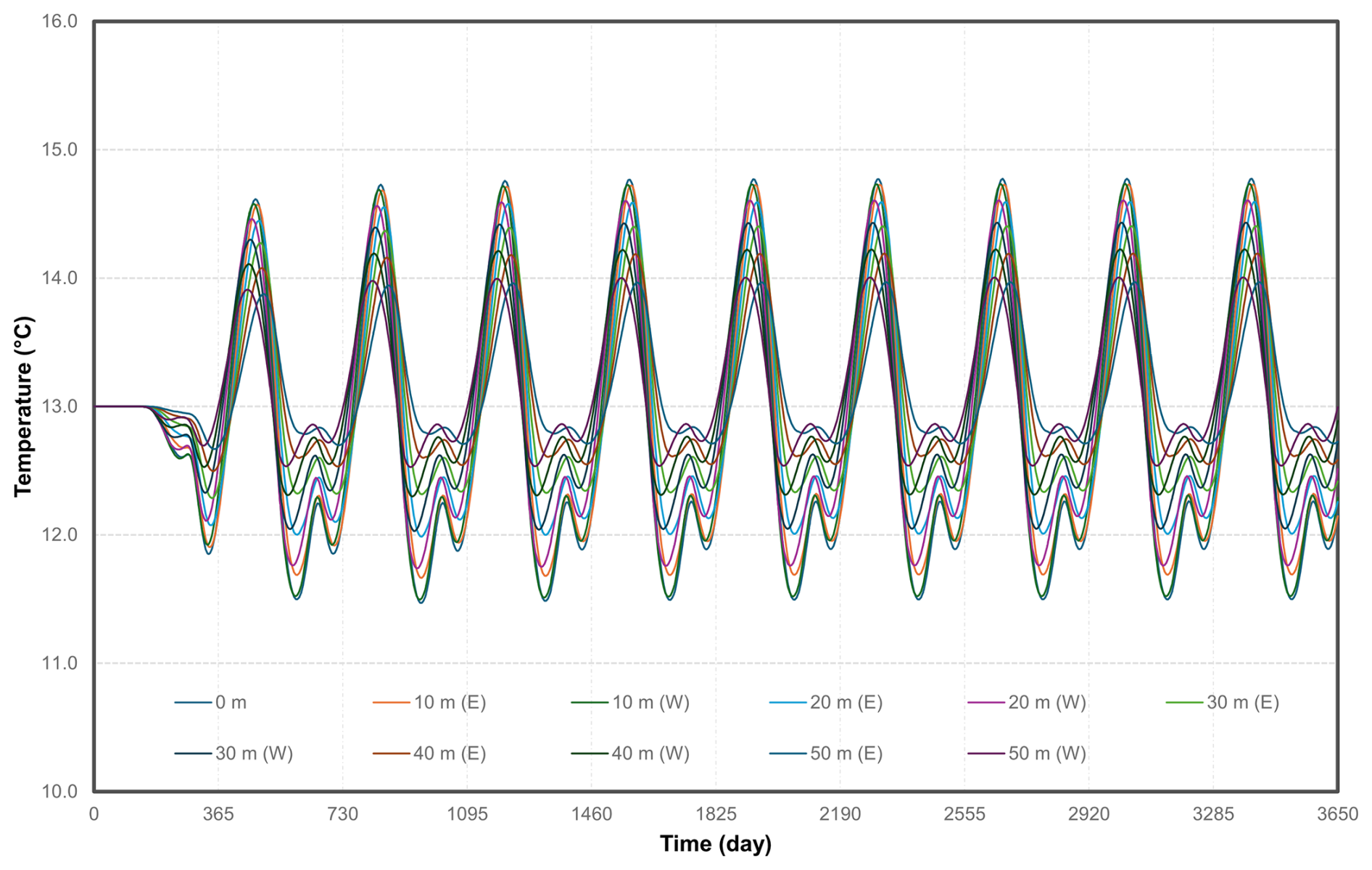
Figure 10 Temperature profiles at the property boundary 0 m and 10, 20, 30, 40, 50 m east and west of the streamline through the extraction well.

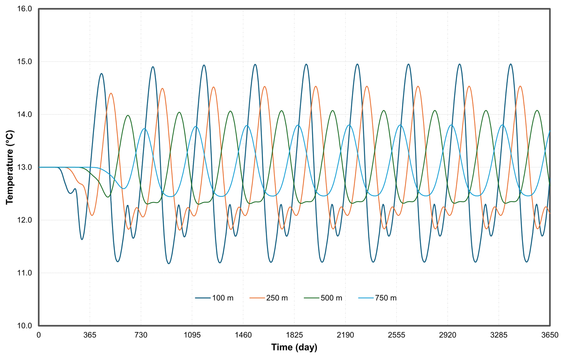
Figure 11 Temperature profiles at distances of 100, 250, 500 and 750 m from the extraction well.

In order to visualise the decay of the plume in the flow direction, the temperature profiles are shown in Fig. 11 at distances of 100, 250, 500 and 750 m along the streamline through the extraction well. From a distance of about 500 m from the extraction well, the temperature limit of ΔT<1 °C is no longer exceeded.

Figure 12 Heat period budget for the 10-year simulation period.

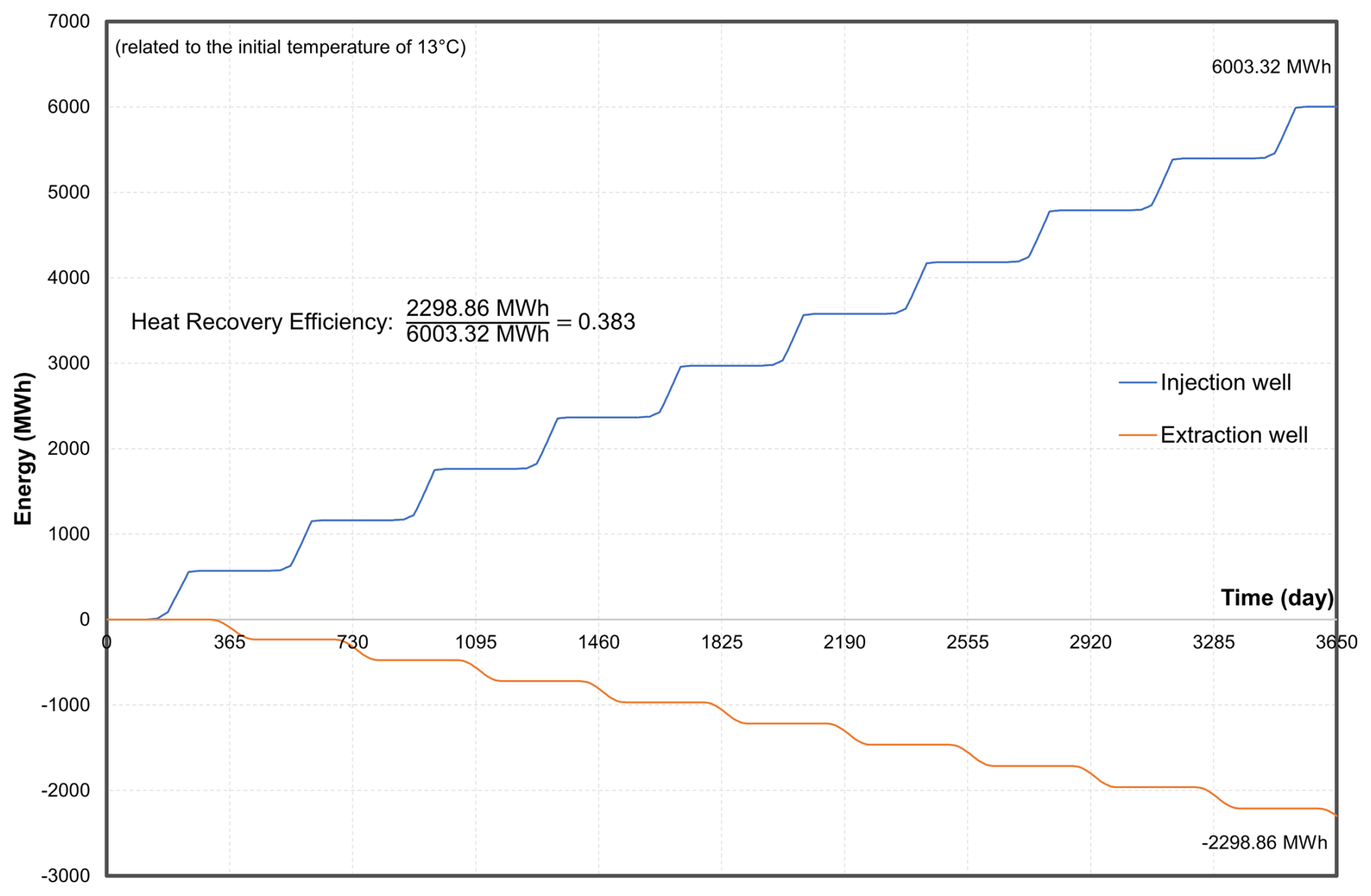
In the numerical model, the unidirectional ATES configuration achieved a thermal recovery efficiency of about 38.3 % over the 10-year simulation period (Fig. 12, corresponding to η_th≈0.383). This value was obtained using Eq. (8) based on the injection and extraction flow rates, the ambient groundwater temperature, and the simulated temperatures at the extraction well.

5 Discussion and outlook

5.1 Model uncertainties

Accuracy of the simulation results is limited by uncertainties in the hydrogeological model. The base of the aquifer in the model was derived from a regional groundwater study and relies in part on interpolation. Considering the complex depositional history of the valley floor, unrecognized paleochannels could exist that would locally increase or decrease the aquifer thickness. Within the project area, hydraulic conductivities were measured via pumping tests and are considered reliable. However, farther from the site, such data are sparse. This lack of information – especially regarding heterogeneities in aquifer properties – makes it difficult to predict the far-field spread of the thermal plume and the associated hydrodynamic dispersion with high confidence.

5.2 Thermal recovery efficiency

By contrast, Silvestri et al. (2025) reported markedly higher recovery rates (55 %–75 %) for unidirectional ATES under idealized conditions. In their simulations, the seasonal pumping followed a perfectly balanced cosine distribution, and the aquifer was assumed homogeneous with constant hydraulic conductivity and transmissivity. In the present case, the climate-driven imbalance between heating and cooling demand means that the thermal plumes from summer and winter are unequal, so a single well spacing cannot fully capture both. This, coupled with natural aquifer heterogeneity, explains the significantly lower recovery efficiency observed in this study. Nevertheless, the unidirectional system still provides substantial energy reuse – whereas a conventional open-loop “pump-and-dump” system has by definition a thermal recovery of zero (since no heat is stored for later use), the modelled unidirectional ATES recovers nearly 40 % of the thermal energy injected in the previous season for useful heating.

5.3 Conceptual Considerations: ATES Definition

The term “unidirectional ATES” was introduced by Silvestri et al. (2025) to describe an open-loop geothermal system with a reversed well scheme as an alternative to the typical one-directional pump-and-dump configuration. The basic idea is to counteract heat loss due to groundwater advection by extracting groundwater from a downstream well and reinjecting it upstream, so that a thermal plume injected in one season can be retrieved in the next. However, classical ATES systems have defining characteristics that set them apart from such one-way configurations. Traditional ATES is an open-loop technology that uses bidirectional well pairs (often termed “warm” and “cold” wells) which alternate between injection and production roles depending on seasonal needs. In other words, thermal energy is actively stored in the aquifer during part of the year (e.g. summer) and later extracted for use in another part of the year (e.g. winter), with the wells switching function between injection and extraction. In a strictly unidirectional open-loop system, by contrast, one well continuously produces groundwater to meet heating/cooling demand and another well continuously injects the thermally spent water (dumping excess heat or cold) without seasonal role reversal. According to Jackson et al. (2024), such one-directional systems do not meet the traditional definition of an ATES, because they lack true long-term thermal storage and reuse of the injected energy. In practice, the design presented in this study blurs the line between these definitions: by aligning the well pair with the natural flow direction and optimizing their distance, a portion of the injected thermal energy is indeed stored in the aquifer and later recovered. Thus, even though the flow is unidirectional at any given time, the system achieves a seasonal storage effect, realizing the principal benefit of an ATES (heat reuse) within a modified operational scheme.

5.4 Comparison with Conventional Open-Loop Systems

A clear advantage of the unidirectional ATES approach is the greatly reduced thermal plume in the aquifer compared to an equivalent conventional open-loop system. The modeling results for the unidirectional case versus a standard open-loop case show that the temperature perturbation in groundwater is much more confined with the unidirectional scheme. For instance, at the downstream property boundary of the project site, the peak groundwater temperature change is on the order of only 2.5 °C in the unidirectional ATES scenario. In contrast, a traditional open-loop configuration produces a significantly larger temperature anomaly at similar distances. By seasonally recapturing the thermal plume instead of allowing it to drift freely, the unidirectional system limits off-site temperature changes to a much smaller magnitude. This mitigation of thermal impacts is crucial for complying with environmental regulations and protecting neighboring groundwater users, and it is what makes a large-scale project feasible in an urban area like Graz.

5.5 Outlook

The project is now transitioning from modeling to real-world implementation. A comprehensive application for water rights for the first phase of the plan has been submitted to the competent authorities. Once approval is obtained, the first pair of wells will be drilled and connected to selected hospital buildings to begin operation. An extensive monitoring phase of approximately two years is planned to follow the commissioning of this initial well pair. During this period, six monitoring wells will be installed to continuously record groundwater levels and temperatures, in order to document the system's hydraulic behavior and thermal evolution in the aquifer. These monitoring stations are strategically positioned, some between the extraction and reinjection wells (to observe the movement and recapture of the thermal plume within the system), and others further downstream at the property boundary (to detect any temperature changes leaving the project site). Data collected from this monitoring program will enable a thorough evaluation of the system's performance and will be used to calibrate the numerical flow and heat transport model (i.e. a thermo-hydraulic calibration under real operating conditions). After this evaluation, the plan is to scale up the installation to the full design capacity: a total of three well pairs with a combined maximum extraction rate of about 180 L s⁻¹. This upscaling will allow the system to supply roughly a peak thermal power of 3.5 MW heating/cooling capacity to the hospital, demonstrating the concept's applicability at the intended project scale.

A fundamental difference to be addressed in future evaluations is the absence of long-term aquifer conditioning in unidirectional ATES. In classical bidirectional ATES systems, flow reversal establishes a “warm” and a “cold” side, leading over time to heating of the aquifer matrix (solid grains). In unidirectional ATES, by contrast, the location of warm and cold zones shifts seasonally, preventing such gradual thermal loading of the solid matrix. This fundamental distinction may have important implications for long-term recovery efficiency and for the sustainable thermal management of the aquifer, and will therefore be a key aspect of the ongoing monitoring and analysis phase.

6 Conclusions

This study presented an evaluation of probably the first unidirectional Aquifer Thermal Energy Storage (ATES) system in Austria, which is being implemented to supply thermal energy to the Hospital Graz South Hospital. The concept involves inverting the conventional well arrangement to align with natural groundwater flow, so that injected thermal plumes are carried downstream by the aquifer and can be recaptured in the following season. Site investigations confirmed that the aquifer has a very high hydraulic conductivity (on the order of $\mathrm{7.5}\times {\mathrm{10}}^{-\mathrm{3}}$ m s⁻¹), which allows a relatively compact installation (three well pairs) to deliver the required peak thermal power of 3.5 MW. A coupled groundwater flow and heat transport model was developed to optimize the system design under these site conditions. The optimal spacing between the extraction and reinjection wells for the first well pair was determined to be approximately 463 m, a distance that maximizes seasonal heat recovery while minimizing off-site thermal effects where minimising thermal effects was crucial.

The simulation results indicate that even without a perfectly balanced seasonal load (due to the predominance of heating over cooling demand in the local climate), the unidirectional ATES greatly reduces thermal dispersion in the aquifer compared to a traditional open-loop system. A big part of the thermal energy injected during the summer cooling season is recovered in the following winter heating season, substantially improving the overall efficiency of the hospital's heating and cooling network. At the same time, thermal anomalies in the aquifer remain largely confined to the project area – the temperature change in groundwater falls below 1 °C at roughly 160 m downstream of the wells, ensuring negligible impact on neighboring water users. These outcomes validate the theoretical promise of the unidirectional ATES concept (as postulated by Silvestri et al., 2025) with practical, site-specific evidence from the model.

In summary, the Graz Süd unidirectional ATES system demonstrates a feasible and effective path for large-scale geothermal energy use in an urban area, particularly under conditions of high ambient groundwater flow that would challenge conventional ATES designs. The system achieves significant utilization of renewable thermal energy and a corresponding reduction in greenhouse gas emissions by replacing a portion of the hospital's fossil-fuelled heating and conventional chiller-based cooling with seasonal aquifer storage. Notably, this is accomplished while maintaining a minimal thermal footprint that adheres to environmental constraints and regulatory requirements. The successful design and planned implementation of this pilot project can pave the way for similar unidirectional ATES applications in other regions where standard ATES configurations might be impractical due to hydrogeological constraints.

The simulation results and site-specific findings at Graz South suggest that the unidirectional ATES (UD-ATES) system is not only feasible at this location but also transferable to other urban and hydrogeologically suitable settings. Key parameters for successful application include moderate to high groundwater velocities (around 1.2 to 5.8 m s⁻¹), sufficient aquifer thickness (5 to 10 m) and hydraulic conductivity (over $\mathrm{5}\times {\mathrm{10}}^{-\mathrm{3}}$ m s⁻¹), and spatial flexibility to achieve optimized well spacing (typically ≥400 m).

The system's effectiveness under unbalanced seasonal loads and natural aquifer heterogeneity demonstrates its robustness beyond idealized conditions. Even with a recovery efficiency of ∼38 %, the UD-ATES markedly outperforms conventional open-loop systems, which lack thermal reuse entirely. Sites with regulatory constraints on thermal impacts or limited space for conventional ATES layouts may particularly benefit from this approach. Analytical predesign methods based on local flow conditions can support initial feasibility assessments before committing to numerical modeling.

These findings support the broader applicability of UD-ATES as a low-impact, high-efficiency alternative for large-scale open loop systems, especially in regions where classical open loop configurations are not viable.

Looking ahead, future work will concentrate on monitoring the system's performance once it is operational and comparing the observed data with the model predictions – an important step to refine the simulation approach and confirm the long-term sustainability of the concept. Additionally, there is potential to expand the system to multiple well pairs (beyond the initial three) and to integrate it with other energy technologies or management strategies (including auxiliary heat dissipation for any excess thermal energy) to further enhance overall efficiency and resilience. The insights gained from this project contribute to the growing field of geothermal energy storage and provide a valuable reference case for harnessing aquifers as safe, efficient, and innovative thermal energy reservoirs.

Appendix A: Operating data and pumping test data in the wells examined

A1 Drinking Water Wells 1 and 2

The two large-diameter shaft wells, Well 1 and Well 2, were tested consecutively. Initially, five pumping stages at a rate of 12.7 L s⁻¹ were conducted in Well 2. At the same time, the water supply for the facility was shut off, but partial water extraction in Well 1 continued in three pumping stages (Fig. A1). The production phase in Well 2 evaluated in Well 1 is shown in Fig. A2.

A2 Well A-H1

The geothermal well A-H1 was operated intermittently during the pumping test period, with peak pumping rates of up to 30 L s⁻¹, causing drawdowns of approximately 0.20 to 0.25 m.

Between operating pauses, three pumping phases – 9 August 2024, 19 August and 20 August 2024 – were conducted over a longer period with quite constant pumping rates ranging between 35.23 and 35.82 L s⁻¹ (Fig. A3). The production phase evaluated in Well A-H1 is shown in Fig. A4.

A3 Well K-JP

The operational pumping in Well K-JP was carried out with a maximum flow rate of 5.08 L s⁻¹. Depending on the duration of the pumping stages, drawdowns between 0.13 and 0.18 m were observed. The longest pumping stages with constant flow rates lasted between 8 and 17 h (Fig. A5). The production phase evaluated in Well K-JP is shown in Fig. A6.

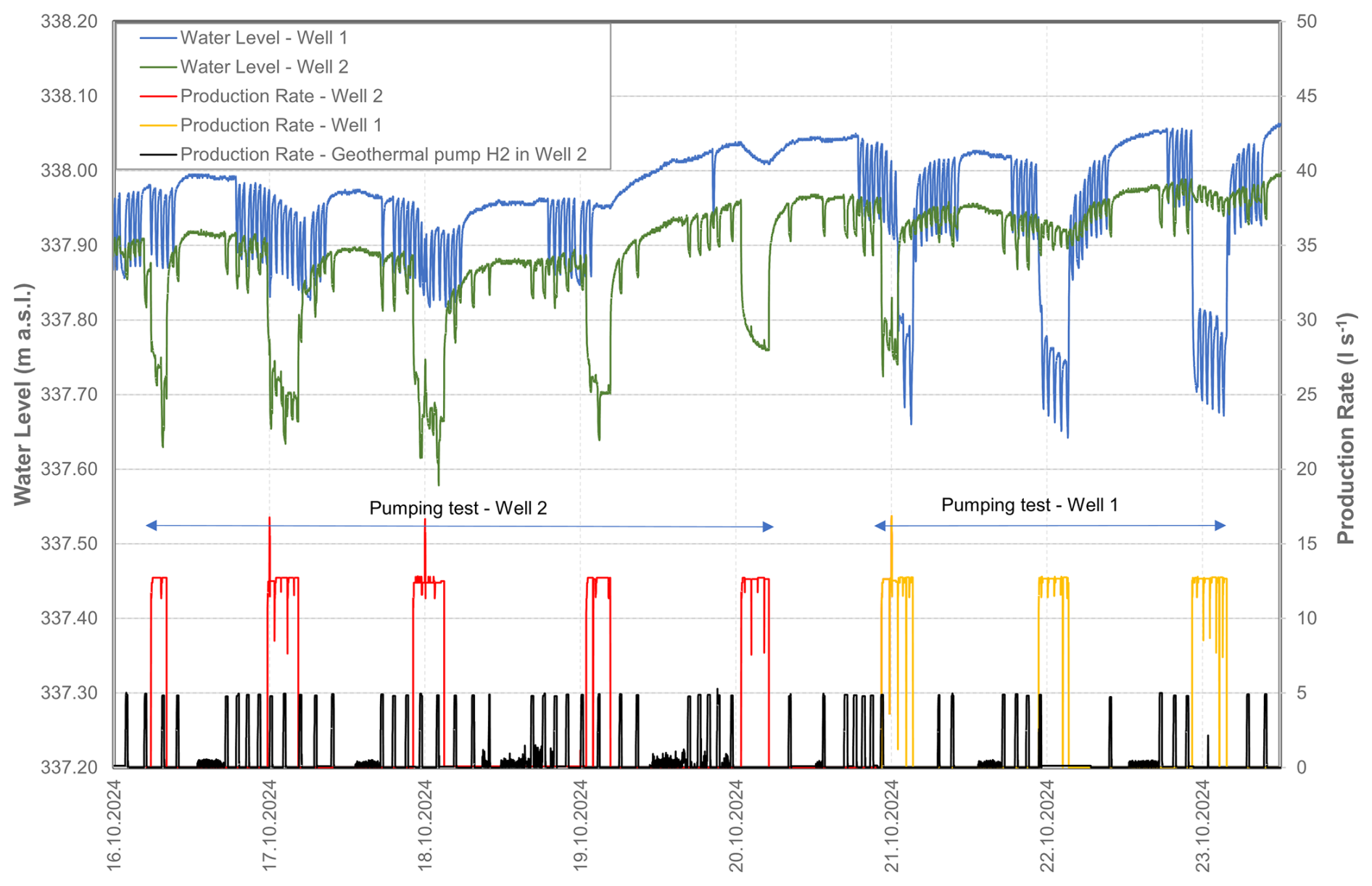
Figure A1 Operational data of Wells 1 and 2 during the observation period. Water level (m a.s.l.) in Well 1, water level (m a.s.l.) in Well 2; production rate (L s⁻¹) of Well 1, production rate (L s⁻¹) of Well 2; production rate (L s⁻¹) of Well H2.

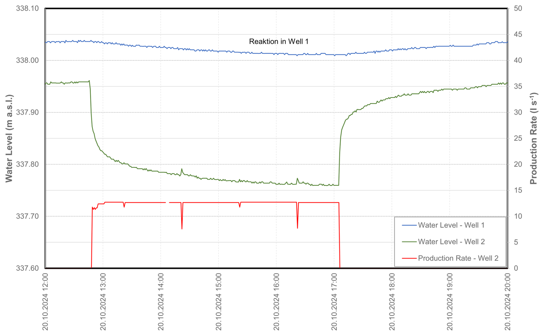
Figure A2 The evaluated production phase in well 2. Water level (m a.s.l.) in Well 1, water level (m a.s.l.) in Well 2; production rate (L s⁻¹) of Well 2 (red line).

Figure A3 Operational data of Well A-H1; water level (m a.s.l.) and production rate (L s⁻¹).

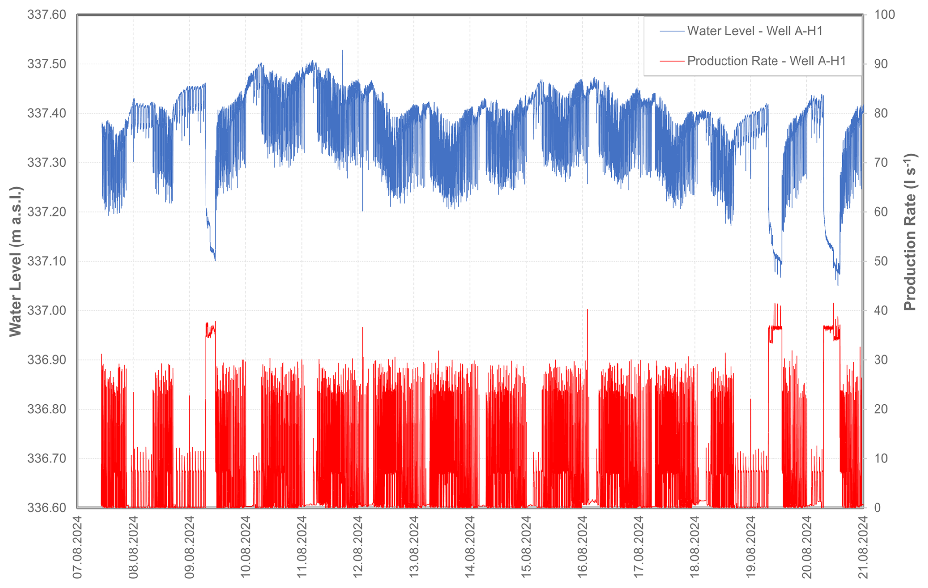
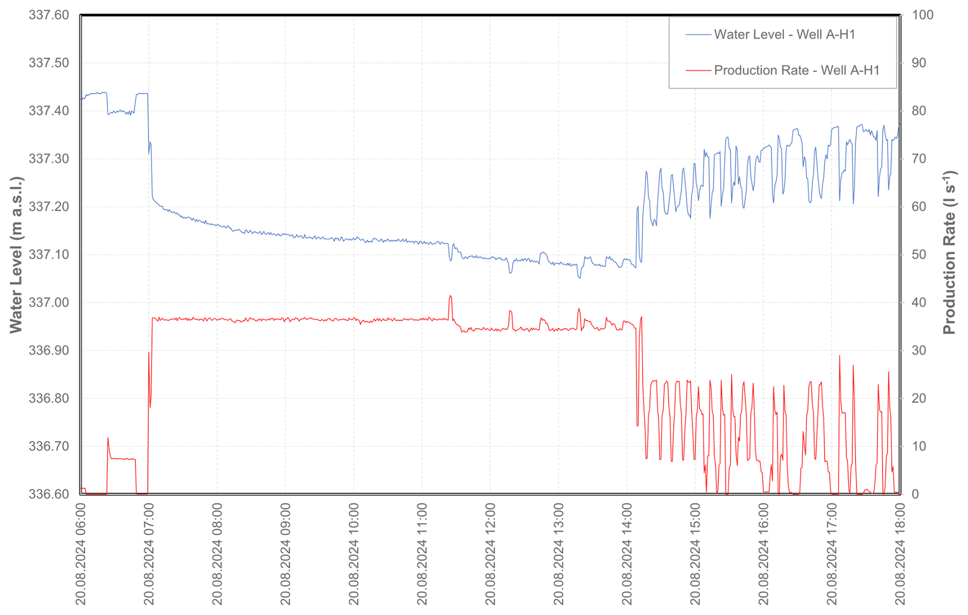
Figure A4 Evaluated production phase in Well A-H1; water level (m a.s.l.) and production rate (L s⁻¹).

Figure A5 Operational data of Well K-JP; water level (m a.s.l.) and production rate (L s⁻¹).

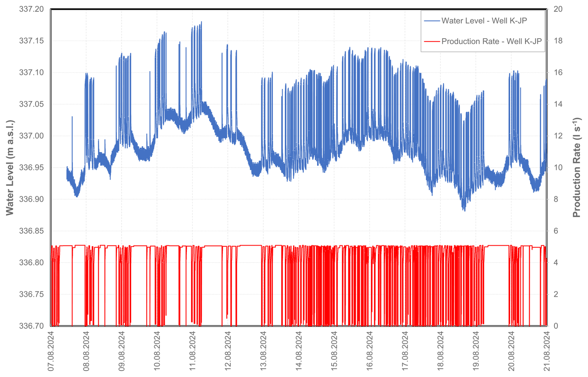
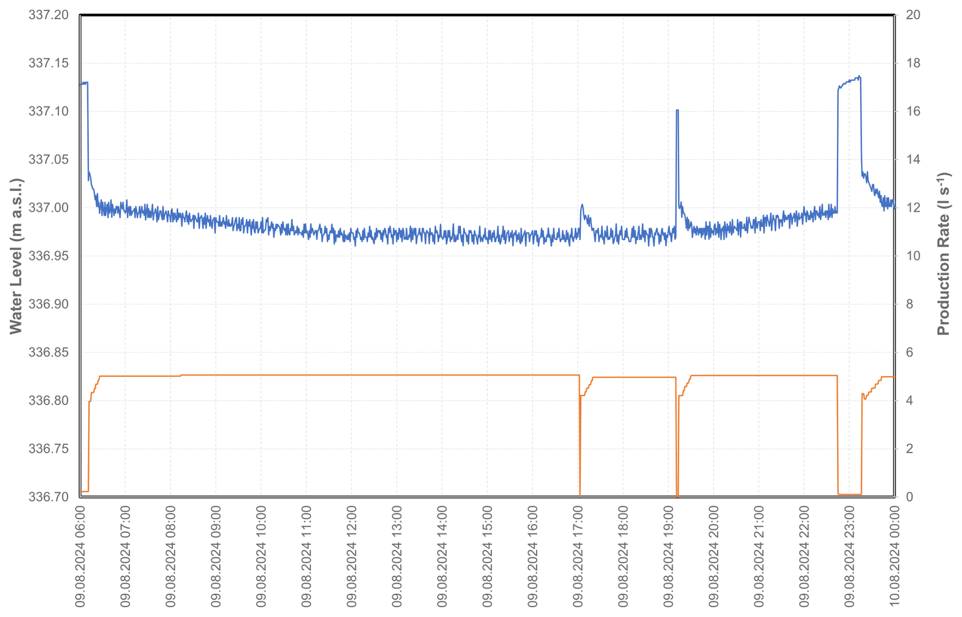
Figure A6 Evaluated production phase in Well K-JP; water level (m a.s.l.) and production rate (L s⁻¹).