Recovery processes in coastal wind farms under sea-breeze conditions

With the rapid growth in offshore wind energy, it is important to understand the dynamics of offshore wind farms. Most of the offshore wind farms are currently installed in coastal regions where they are often affected by sea-breezes. In this work, we quantitatively study the recovery processes for coastal wind farms under sea-breeze conditions. We use a modified Borne's method to identify sea breeze days off the west coast of India in the Arabian Sea. For the identified sea breeze days, we simulate a hypothetical wind farm covering 50×50 km² area using the Weather Research and Forecasting (WRF) model driven by realistic initial and boundary conditions. We use three wind farm layouts with the turbines spaced 0.5, 1, and 2 km apart. The results show an interesting power generation pattern with a peak at the upwind edge and another peak at the downwind edge due to sea breeze. Wind farms affect the circulation patterns, but the effects of these modifications are very weak compared to the sea breezes. Vertical recovery is the dominant factor with more than half of the momentum extracted by wind turbines being replenished by vertical turbulent mixing. However, horizontal recovery can also play a strong role for sparsely packed wind farms. Horizontal recovery is stronger at the edges where the wind speeds are higher whereas vertical recovery is stronger in the interior of the wind farms. This is one of the first studies to examine replenishment processes in offshore wind farms under sea breeze conditions. It can play an important role in advancing our understanding wind farm-atmospheric boundary layer interactions.

1 Introduction

Wind turbines extract momentum from the atmosphere to convert it into electricity. The momentum extracted by the wind turbines is replenished by the transport of higher momentum air from aloft (vertical recovery) and from the lateral edges (horizontal recovery) almost immediately (Calaf et al., 2010; Cortina et al., 2020; Gupta and Baidya Roy, 2021). Cortina et al. (2020) found that in the finite-sized wind farms under neutral conditions, horizontal recovery dominates for the first upwind row of turbines and vertical recovery dominates for the last row with a smooth transition in between. Gupta and Baidya Roy (2021) concluded that the vertical recovery is the dominant factor in replenishment for all the wind speed ranges and wind farm configuration for a finite sized wind farm. They also found similar spatial recovery patterns to that of Cortina et al. (2020) for densely packed deep offshore wind farms. So far, all the work on recovery in finite-sized wind farms have been done either for onshore wind farms (Cortina et al., 2020) or for deep offshore wind farms (Gupta and Baidya Roy, 2021). However, the current installations of offshore wind farms are mostly near the coast. These coastal wind farms are often affected by sea breeze. Various studies (Seroka et al., 2018; Kumar et al., 2021) have identified the importance of sea-breeze for coastal wind farms. However, none of the studies done earlier have investigated the recovery processes in coastal wind farms under sea breeze conditions.

The objective of this study is to quantitatively understand the recovery processes in a hypothetical coastal wind farm under sea breeze conditions using numerical experiments. The wind farm is located in the Arabian sea off the west coast of India, near Mumbai. Sea breezes occur quite frequently in this region (Lei et al., 2008; Kumar et al., 2021). To the best of our knowledge, this is the first study to explore recovery processes in coastal wind farms.

2 Methodology

2.1 Modelling approach

The study uses a numerical modelling approach by conducting simulations with the Weather Research and Forecasting (WRF) model that is equipped with a wind turbine parameterization. The numerical simulations are conducted in two steps. First, we conducted simulations using the WRF model with the wind turbine parameterization turned off to generate a meteorological dataset for 4 summer months. This is needed because a high-resolution network of observation stations required for identifying mesoscale circulations like sea breezes is not available in that region. The simulated meteorological dataset was used to identify sea breeze days using the Borne's method (Borne et al., 1998). The outcome was evaluated using Meteorological Terminal Aviation Routine Weather Report (METAR) data from an Integrated Surface Database station located at Mumbai Airport (NOAA-NCEI, 2001). Next, we conducted simulations for the sea breeze days with the wind turbine parameterization turned on to simulate the behaviour of the hypothetical wind farm.

Section 2.2 describes the WRF model and the configuration used in the simulations to generate the meteorological data. Section 2.3 describes the Borne's method. Section 2.4 describes the WRF wind turbine parameterization and the configuration used to simulate the hypothetical wind farm for the sea breeze days identified in Sect. 2.3. Section 2.5 covers the formulae used in calculation of recovery and fluxes.

2.2 WRF model configuration for sea breeze identification

The WRF model version 4.2.1 was used for conducting numerical simulations. WRF is a state-of-the-art mesoscale numerical model that solves the conservation equations for velocity, mass, energy, and scalars. The horizontal grid is staggered using Arkawa C-grid technique (Mesinger and Arakawa, 1976) and the vertical coordinate system is terrain-following and is based on dry hydrostatic pressure levels. Various physics parameterization schemes are available in WRF to represent atmospheric radiative and microphysical process. Skamarock et al. (2019) gives further details regarding the WRF model.

The study area is the Arabian Sea coast near Mumbai (Fig. 1). This region is high in wind resources (Harikumar et al., 2011) where sea breezes are a common occurrence (Lei et al., 2008; Kumar et al., 2021). Figure 1 shows the WRF simulation domains. The innermost domain is 150 km×150 km and discretized with a rectangular Cartesian grid with 1 km spacing. This domain was nested within two coarser domains of size: 450 km×450 km and 1350 km×1350 km, discretized with 3 and 9 km spacings, respectively. Two-way nesting technique was used for the simulations. The model vertical grid used 61 levels from the surface to the model top at 100 hPa. The vertical spacing was kept finer in the lower layers with at least 7 levels till 150 m for better resolution of boundary layer processes. The horizontal Turbulent Kinetic Energy (TKE) advection was kept “on” for all the simulations.

The study period was two summer months – April and May – for the years 2018 and 2019. April and May are the hottest months in the study region (Kale and Joshi, 2014). Therefore, we expect the land-sea temperature gradient to be high and consequently there is a high probability of sea breeze formation during these months. The model was initialized at 05:30 Indian Standard Time (IST, 00:00 UTC) of each month and run continuously for one entire month. The initial and atmospheric lateral boundary conditions were obtained from the National Centers for Environmental Prediction Final Operational Global Analyses dataset (National Centers for Environmental Prediction et al., 2018) data sets. Physics parameterization schemes used for the simulations are shown in Table 1. The results of these simulations, in particular, the wind speeds and direction at 700 hPa and 10 m, and temperature at 2 m were used as input to the Borne's algorithm to identify the sea breeze days.

Table 1 Physics settings used in WRF simulations.

2.3 Identification of sea breeze days

Borne et al. (1998) developed a novel method that involves six filters to characterize and identify sea-breeze days. Meteorological conditions at a particular site/region on a particular day must pass through six filters for that day to be characterized as a sea breeze day. The six filters and how they were implemented in this study are described below.

1. No rapid change in synoptic conditions in terms of wind direction: days when the wind direction at 700 hPa changes more than 90^∘ during 24 h of time slab were excluded. The 24 h of time slab was taken from 13:00 IST previous day to 13:00 IST on the actual day.

2. No rapid change in synoptic conditions in terms of wind speed: days when the changes in synoptic wind speed at the 700 hPa level is higher than 6 m s⁻¹ during 12 h of time slab were excluded. The 12 h of time slab was considered from 01:00 to 13:00 IST.

3. Exclude days when the synoptic wind speed is very strong: days with wind speeds at 700 hPa and at 13:00 IST higher that 11 m s⁻¹ were excluded.

4. Exclude days when the sea to land temperature difference is not strong enough to develop a sea breeze: days where land-atmosphere temperature difference was less than 3 ^∘C were excluded.

5. Exclude days when there is no quick change in the surface wind direction for the hours when sea breeze formation is favourable: days with change in wind direction <30^∘ during the hours from (sunrise+1 h) to (sunset−5 h) are excluded.

6. Exclude the days when strong veering conditions are prevalent but are not because of sea breeze. Additionally, in this filter the sea breeze days with very short duration time are also excluded: days where $D_{\mathrm{peak}}/D_{\mathrm{5}\mathrm{mean}}<\mathrm{6}$ during the hours from sunrise+1 h to sunset are excluded, where D_peak is the change in surface wind direction and D_5mean is the average of the hourly changes in surface wind direction in the 5 h following the D_peak.

We modified this technique by adding a seventh filter where we excluded the days when the wind direction does not become perpendicular to the coastline during the period when the sea breeze formation is favourable. This filter was added because it is well known that sea breezes flow perpendicular to the coastline (Azorin-Mollina et al., 2011).

Based on the above algorithm, we identified the 5 sea breeze days out of the 4-month study period. The details of the sea-breeze days that are identified and their validation against METAR data are given in Sect. 3.1. We conducted numerical simulations with the WRF wind farm parameterization on these days to study the behaviour of a hypothetical coastal wind farm under sea-breeze conditions.

2.4 Model configuration for wind farm simulations

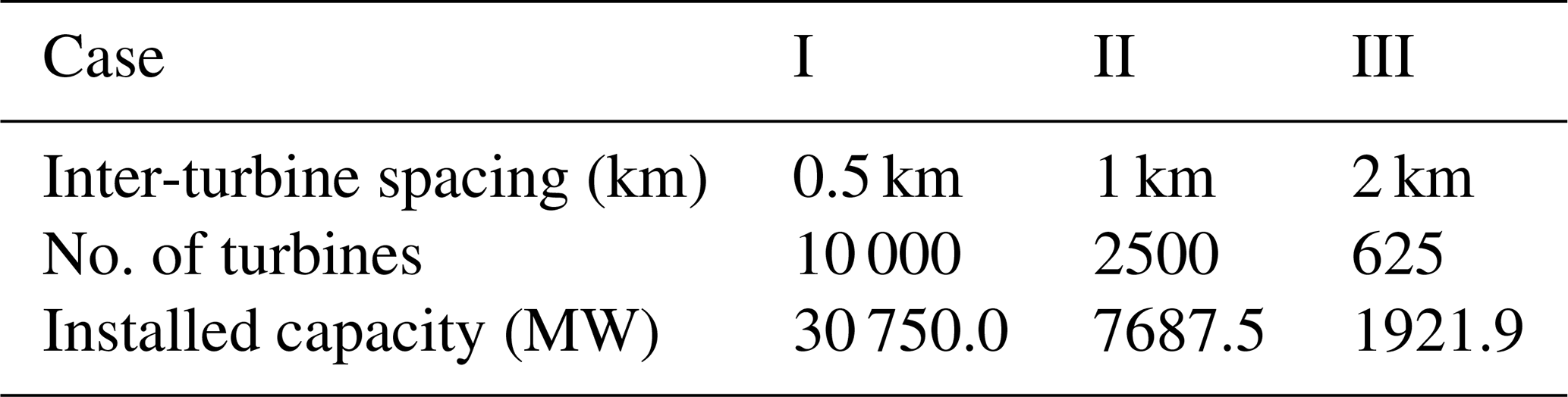
The WRF model was used to simulate the behaviour of coastal wind farms. The same configuration described in Sect. 2.2 was used for these simulations except for two differences. First, a hypothetical wind farm was placed over a 50 km×50 km area 1 km away from the coast at the centre of domain 3 (Fig. 1). In the WRF model, wind turbines are parameterized as momentum sink and TKE source (Fitch et al., 2012). The wind farms consist of 3.075 MW turbines with the same specifications as Gupta and Baidya Roy (2021). The horizontal TKE advection switch was turned “on” and the correction factor for TKE coefficient was set to one (Gupta and Baidya Roy, 2021; Larsén and Fischereit, 2021). Three wind farm layouts based on different inter-turbine spacings are studied. The characteristics of the layouts are described in Table 2.

Table 2 Wind farm layout characteristics.

The second difference is that instead of 4 months, we simulated the wind farm behaviour for only the sea breeze days identified in Sect. 2.3. For each sea breeze day, we conducted two simulations:

1. A 72 h wind farm (WF) simulation with the wind turbine parameterization turned on. This simulation was initialized at 05:30 IST of the day prior to the sea breeze day and was run for 3 d. However, the first 24 h were discarded as spin up.

2. A 72 h control (CTRL) simulation similar to the WF simulation but with the wind turbine parameterization turned off. We decided to conduct the CTRL simulations instead of using the simulations from Sect. 2.2 to ensure that the model is initialised at the same time for both CTRL and WF cases.

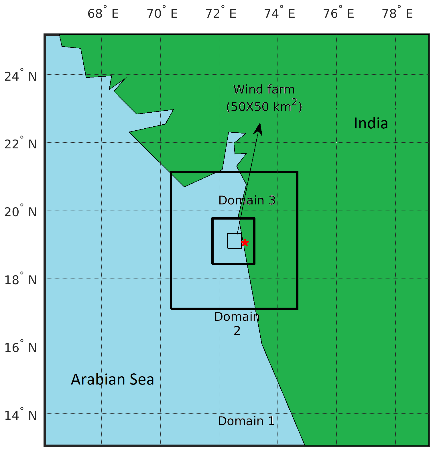
Figure 1 WRF simulation domains showing the location of the 50 km×50 km wind farm within domain 3. The red star shows the METAR station location at Mumbai airport.

2.5 Quantification of fluxes, recovery, and momentum loss rate quantification

Mesoscale fluxes are calculated as per the formulations given by Avissar and Chen (1993). The vertical mesoscale kinematic flux of the zonal momentum (u) and the meridional momentum (v) are given by:

$$\begin{array}{}\text{(1)}& {\displaystyle }U{W}_{\mathrm{meso}}=\left(u-\stackrel{\mathrm{‾}}{u}\right)\left(w-\stackrel{\mathrm{‾}}{w}\right),\text{(2)}& {\displaystyle }V{W}_{\mathrm{meso}}=\left(v-\stackrel{\mathrm{‾}}{v}\right)\left(w-\stackrel{\mathrm{‾}}{w}\right),\end{array}$$

where $u(k,i,j)$, $v(k,i,j)$, and $w(k,i,j)$ are grid resolved zonal, meridional, and vertical velocities, respectively. k, i, j are the model grid points in z, x and y directions, respectively. The overhead bar on the velocities represents the spatial average taken over domain 3 from WRF simulations (Fig. 1). The microscale kinematic fluxes of the zonal and meridional momentums are $u{}^{\prime }w{}^{\prime }(k,i,j)$ and $v{}^{\prime }w{}^{\prime }(k,i,j)$, which are calculated by the MYNN scheme.

Vertical recovery is calculated as the difference in the vertical turbulent flux divergence between the WF and CTRL (WF-CTRL) cases. The corresponding equation is:

$$\begin{array}{}\text{(3)}& \begin{array}{rl}& \text{Vertical Recovery}={\left[-\left({\displaystyle \frac{\partial u{}^{\prime }w{}^{\prime }}{\partial z}}\right)\widehat{i}-\left({\displaystyle \frac{\partial v{}^{\prime }w{}^{\prime }}{\partial z}}\right)\widehat{j}\right]}_{\mathrm{WF}}\\ & -{\left[-\left({\displaystyle \frac{\partial u{}^{\prime }w{}^{\prime }}{\partial z}}\right)\widehat{i}-\left({\displaystyle \frac{\partial v{}^{\prime }w{}^{\prime }}{\partial z}}\right)\widehat{j}\right]}_{\mathrm{CTRL}}.\end{array}\end{array}$$

Here, $u{}^{\prime }w{}^{\prime }$ and $v{}^{\prime }w{}^{\prime }$ are the vertical kinematic turbulent flux of the zonal and meridional momentums and $\widehat{i}$ and $\widehat{j}$ are unit vectors in the zonal (x) and meridional (y) directions, respectively, which are calculated by the MYNN scheme at the model grid points. The flux difference is taken in vertical direction (z) between the heights of 28 and 140 m, that are the lower and upper wind turbine blade tip heights, respectively.

Horizontal recovery is represented by the difference (WF-CTRL) in mean momentum advection. The corresponding equation is:

$$\begin{array}{}\text{(4)}& \begin{array}{rl}& \text{Horizontal Recovery}\\ & ={\left[\left(-u_{\mathrm{h}}{\displaystyle \frac{\partial u_{\mathrm{h}}}{\partial x}}-v_{\mathrm{h}}{\displaystyle \frac{\partial u_{\mathrm{h}}}{\partial y}}\right)\widehat{i}+\left(-u_{\mathrm{h}}{\displaystyle \frac{\partial v_{\mathrm{h}}}{\partial x}}-v_{\mathrm{h}}{\displaystyle \frac{\partial v_{\mathrm{h}}}{\partial y}}\right)\widehat{j}\right]}_{\mathrm{WF}}\\ & -{\left[\left(-u_{\mathrm{h}}{\displaystyle \frac{\partial u_{\mathrm{h}}}{\partial x}}-v_{\mathrm{h}}{\displaystyle \frac{\partial u_{\mathrm{h}}}{\partial y}}\right)\widehat{i}+\left(-u_{\mathrm{h}}{\displaystyle \frac{\partial v_{\mathrm{h}}}{\partial x}}-v_{\mathrm{h}}{\displaystyle \frac{\partial v_{\mathrm{h}}}{\partial y}}\right)\widehat{j}\right]}_{\mathrm{CTRL}}.\end{array}\end{array}$$

Here, u_h and v_h are the hub-height wind speeds in the zonal (x) and meridional (y) directions, respectively. The gradients are calculated using central finite differencing method. The vector difference in Eqs. (3) and (4) are projected on the prominent wind direction from the CTRL case.

Momentum loss rate is defined as per the formulation given in Fitch et al. (2012).

$$\begin{array}{}\text{(5)}& {\left.{\displaystyle \frac{\partial \left|V\right|}{\partial t}}\right|}_{(k,i,j)}=-{\displaystyle \frac{\frac{\mathrm{1}}{\mathrm{2}}{N}_{\mathrm{t}}(i,j)C_{\mathrm{T}}{\left|V(k,i,j)\right|}^{\mathrm{2}}A(k,i,j)}{z(k+\mathrm{1},i,j)-z(k,i,j)}}.\end{array}$$

Here, $V(k,i,j)=\left[u(k,i,j),v(k,i,j)\right]$ is the horizontal wind velocity (m s⁻¹), N_t(i,j) is number of turbines per square metre (m⁻²) for the grid cell (i,j), C_T is turbine thrust coefficient which is dependent on V at hub-height, $A(k,i,j)$ is cross-sectional rotor area (m²), $z(k,i,j)$ is height (m) of level k.

The momentum loss rate is also projected along the prominent wind direction from the CTRL case for it to be consistent with the recovery terms.

3 Results

3.1 Sea-breeze days validation using METAR data

Five sea breeze days were identified by applying the 7-filter modified Borne's method on the meteorological dataset over the study area. The 5 d are: 4 May 2018, 7, 8, 9, and 21 April 2019. The simulations are evaluated against observations from a weather station located at 19.088686^∘ N, 72.867919^∘ E and 11.27 m height. The simulated wind speed and wind direction from the WRF grid cell at that location linearly interpolated to 11.27 m height is compared with the observations (Fig. 2). The simulations match the observations quite well with a correlation of 0.69. The figure shows strong signs of sea breezes with a sharp increase in wind speeds after 12:00 IST every day in both observations and model results. However, the increase occurs more gradually and slightly earlier in the simulations compared to the observations. There is also a reversal in the wind direction of almost 180^∘ from early morning time to the afternoon.

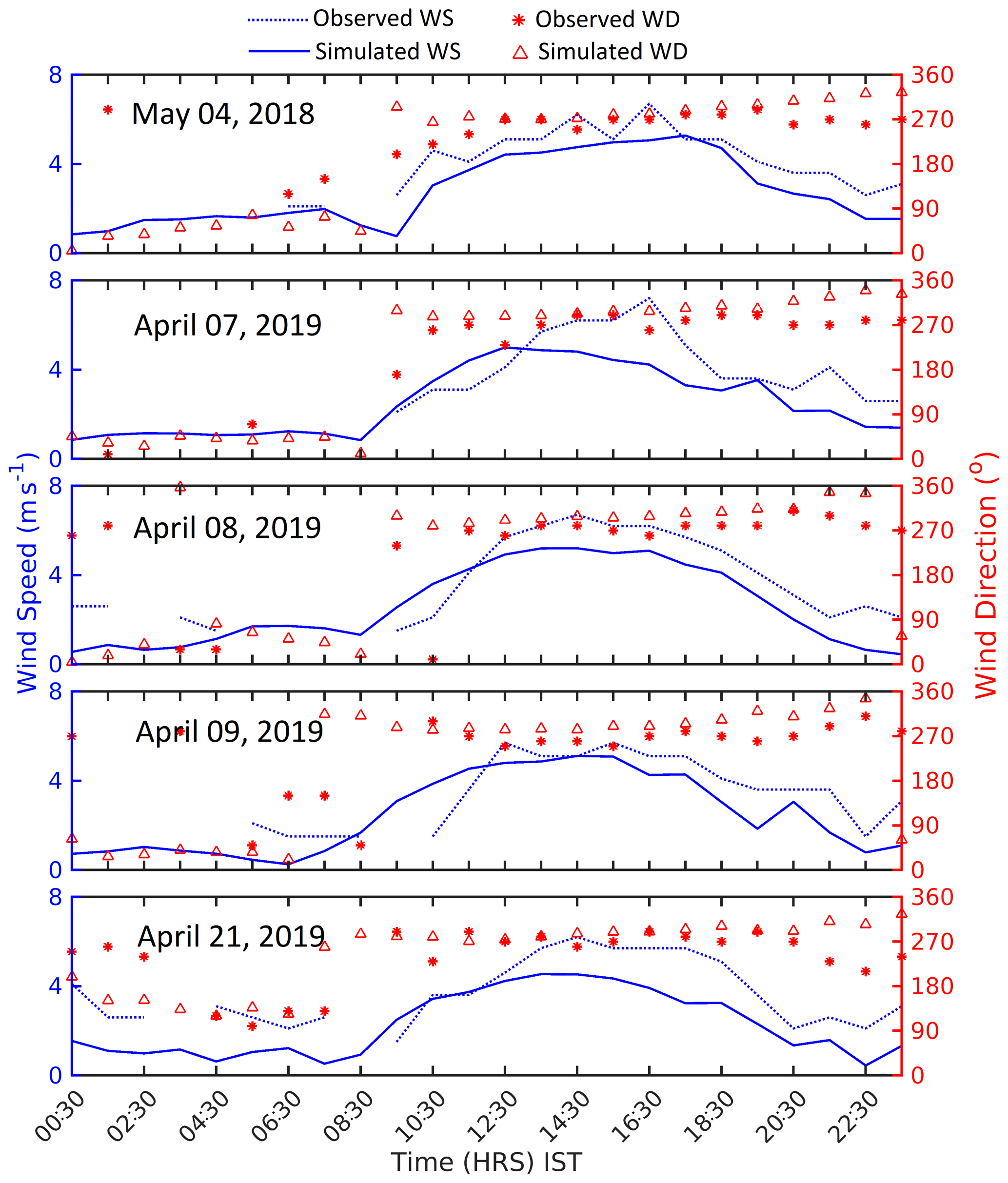
Figure 2 Time series of simulated (CTRL case) and observed wind speed (WS) and wind direction (WD) at 11.27 m for the 5 sea breeze days.

3.2 Power production under sea breeze conditions

The power production for 5 sea breeze days, averaged over the sea breeze hours from 12:30 IST to 17:30 IST for different wind farm layouts are shown in Fig. 3. Power production follows an interesting spatial pattern under sea breeze conditions. The winds are predominantly westerly during the study period with a 274.3^∘ wind direction averaged over the sea breeze hours. The power production is high at the western upwind edge of the wind farm, and thereafter it decreases because of wake effects. However, the power production again increases towards the eastern downwind edge. This is because of the increase in wind speeds as the wind approaches land due to sea breeze formation (Figs. 4 and 5). This contrasts with the earlier study by Gupta and Baidya Roy (2021), where the power production monotonically decreased from the upwind edge to the downwind edge because of wake effects. The earlier study mentioned above was for a deep offshore wind farm where there were no sea breezes.

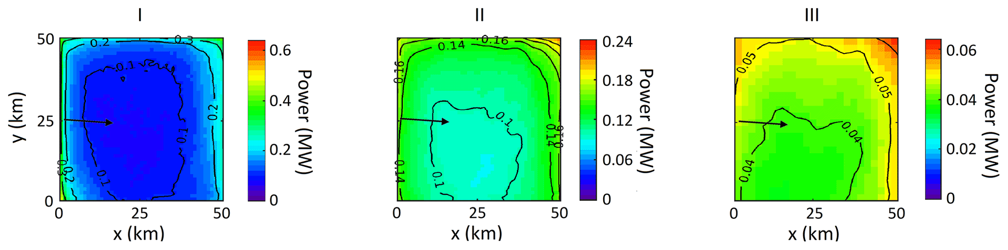
Figure 3 Averaged power (MW) generated in the WF cases: I, II and III. Power is averaged over 5 sea-breeze days for 12:30 to 17:30 IST. The black arrow represents the prominent wind direction. It is to be noted here that colorbars for cases I, II and III have different upper limits.

Figure 4 (a) Wind anomalies and (b) power production for 7 April 2019, at (i) 12:30 IST, (ii) 14:30 IST, and (iii) 15:30 IST.

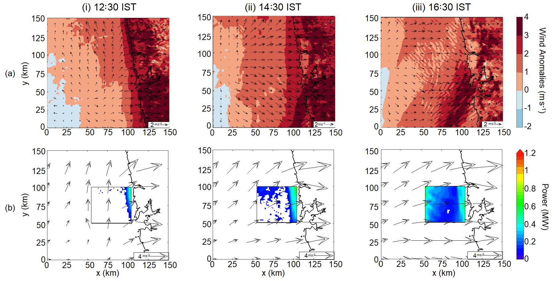
Figure 5 (a) Wind anomalies and (b) power production for 4 May 2018 at (i) 12:30 IST, (ii) 14:30 IST, and (iii) 16:30 IST.

The total power production of the wind farm averaged over sea breeze hours for 5 d are 0.344, 0.29, and 0.11 GW for cases I, II, and III, respectively (Table 3). This decrease in power production from case I to case III is because the installed capacity decrease from case I to case III. However, the wind farm efficiency increases from case I at 16 % to case III at 79 %. This is because of the decrease in wake effects as the inter-turbine distance increases.

Table 3 Power generation (MW) and efficiency (%) for different wind farm cases. Power and efficiency are averaged over 5 sea-breeze days for 12:30 to 17:30 IST.

There is a strong spatial correlation between sea breeze and power production. To give readers a flavour of this effect, we plot the co-evolution of wind speed anomalies from the CTRL simulation and power production from the WF simulation for case I on 7 April 2019 (Fig. 4) and 4 May 2018 (Fig. 5). 7 April 2019 represents a typical case where the winds are westerly throughout but 4 May 2018, is an atypical case with the winds veering strongly during the evolution of the sea breeze. The wind speed anomaly is calculated by subtracting the domain average wind speed from each grid point. Thus, the effects of synoptic-scale phenomena are removed and only the mesoscale signal is present (Avissar and Chen, 1993). Figures 4a.i and 5a.i show that the sea breeze starts forming at 12:30 IST. As the wind approaches land, the speed increases and the direction becomes perpendicular to the coast. The sea breeze is the strongest at around 15:30 IST on 7 April 2019 (Fig. 4a.iii) and 16:30 IST on 4 May 2018 (Fig. 5a.iii) respectively. At 12:30 IST, as the sea breeze starts forming, power is only generated along the eastern edge of the wind farm (Figs. 4b.i and 5b.i). At the western edge, the winds are weak (<3 m s⁻¹) and no power is generated. At 15:30 IST on 7 April 2019 (Fig. 4b.iii) and 16:30 IST on 4 May 2018 (Fig. 5b.iii), when the offshore extent of the sea breeze is maximum and the sea breeze effect is strongest, two peaks in the power generation, both at upwind and downwind edge of the wind farm can be clearly seen. Other cases also depict similar spatial correlation between wind speed anomalies and power production, but they are not discussed in detail due to space constraints.

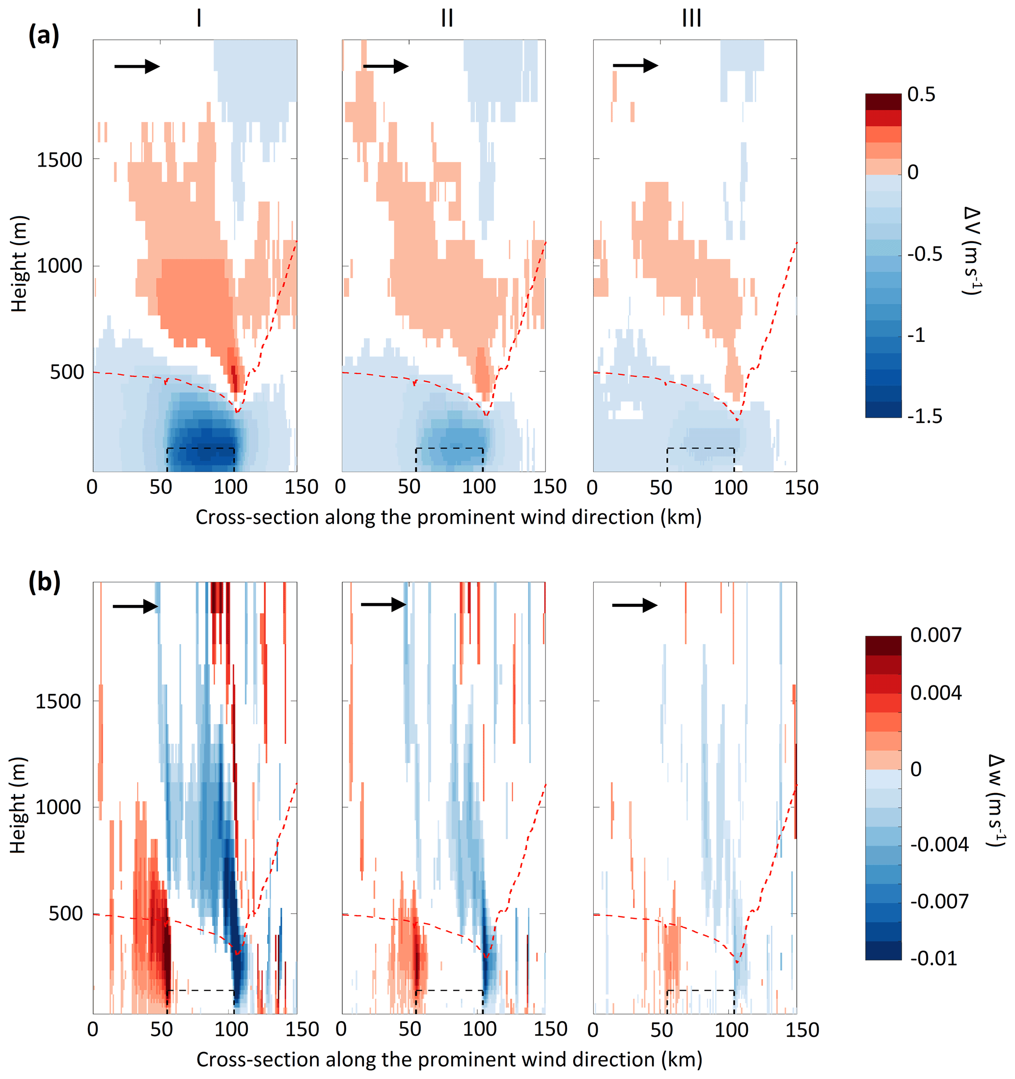
Figure 6 Difference (WF-CTRL) in (a) horizontal wind velocities, ΔV (m s⁻¹) and, (b) vertical wind velocity, Δw (m s⁻¹) on a vertical cross-section along the predominant wind direction for (I) case: I, (II) case II, and (III) case III. Only the statistically significant differences (p<0.01) are shown here. The white-colored regions represent areas where the differences are not significant. The black dashed box depicts the wind farm cross-section. The red dashed line depicts ABL height in the corresponding WF case. The black arrow represents the prominent wind direction. Difference in wind velocities is averaged over 5 sea-breeze days for 12:30 to 17:30 IST.

3.3 Circulation Patterns and fluxes around a wind farm under sea breeze conditions

Figure 6 shows the circulation patterns around a wind farm under sea breeze conditions. There are a few interesting features that can be noticed in the circulation patterns. First, there is a reduction in horizontal wind velocity up to 1.5 m s⁻¹ within the wind farms due to wake effects. The second feature is a clearly visible wake that extends vertically up to 500 m and horizontally between 20–40 km downwind of the wind farms. This wake length is much smaller compared to the deep offshore wind farms of similar sizes and installed capacities simulated by Gupta and Baidya Roy (2021). This is because the wind farms in the current study are only 1 km away from the coast and the wind farm wakes occur mostly over the land where they get dissipated faster due to higher roughness length. Finally, there is a strong signal of modification of the circulation pattern over the wind farm. As the atmospheric flow approaches the wind farm from the west, it slows down due to blockage effect (Bleeg et al., 2018; Porté-Agel et al., 2020). The reduction in upwind horizontal wind velocities is up to 0.5 m s⁻¹ (Fig. 6a). A part of the incoming flow passes through the wind farm while the rest gets lifted upwards as seen in the updrafts at the upwind edge (Fig. 6b). The lifted flow then flows over the wind farm as evident in the increase in horizontal velocity aloft by up to 0.5 m s⁻¹. After crossing the wind farm, the lifted flow descends with downdrafts up to 0.01 m s⁻¹ at the downwind edge of the wind farms.

Figure 7 shows the difference in mesoscale and microscale fluxes averaged for the wind farm for the sea breeze hours. The change in mesoscale fluxes due to wind farm in case of sea breeze is minimal. The lack of any signal in mesoscale fluxes despite the distinct change in the circulation pattern around the wind farm appears to be counterintuitive. This occurs perhaps because there is already a strong mesoscale sea breeze circulation with wind speeds (11.27 m) up to 4 m s⁻¹ operating in the study domain. The wind farm-induced mesoscale circulations with wind speeds up to 0.5 m s⁻¹ are about an order of magnitude weaker than the sea breezes. That is why they do not have a strongly discernible impact on mesoscale transport processes in the domain.

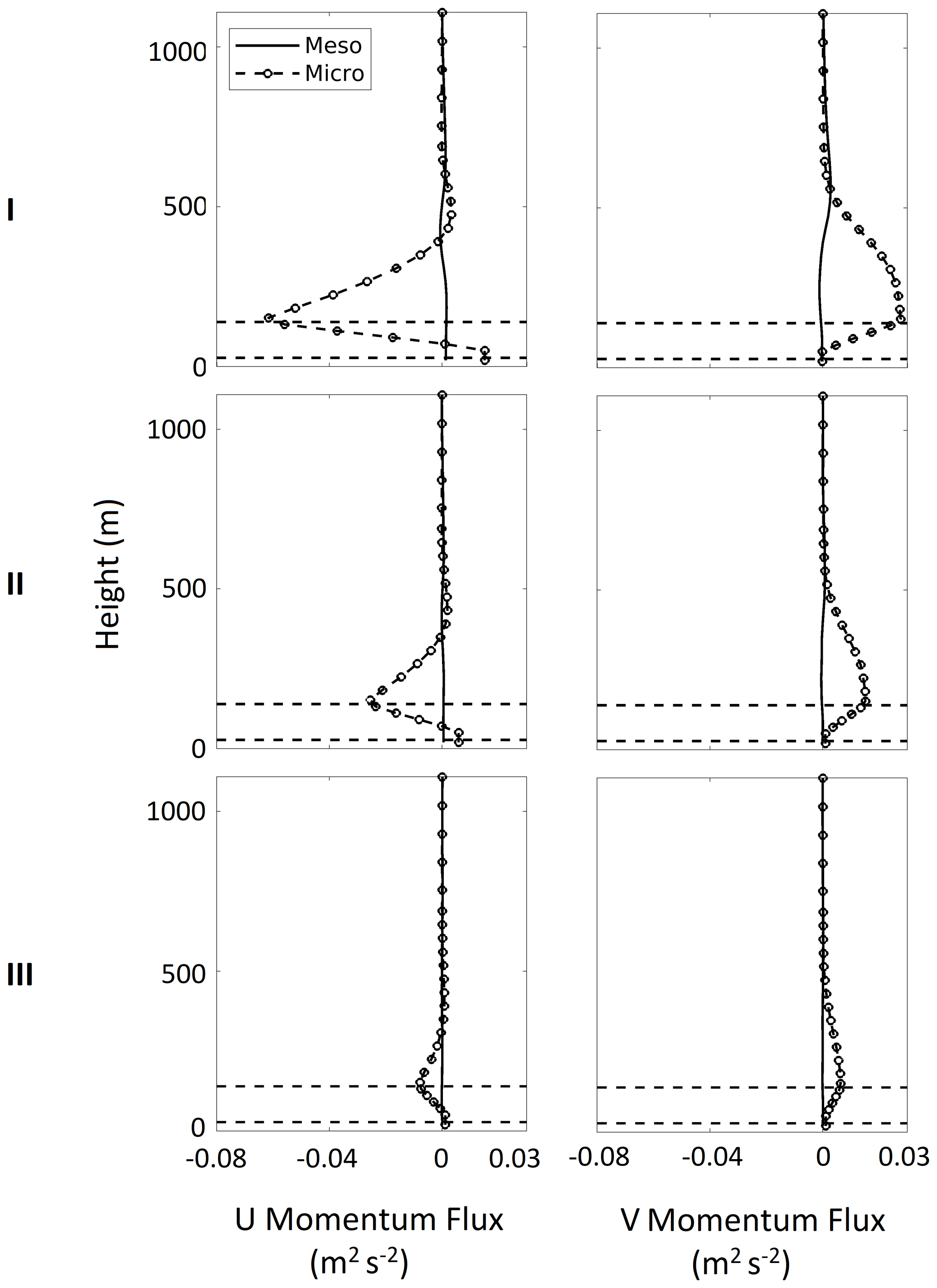
Figure 7 Difference (WF-CTRL) in vertical profiles of mesoscale (solid line), and microscale fluxes (- -o- -) averaged over the wind farm and 5 sea-breeze days for 12:30 to 17:30 IST, for different cases. Horizontal black dotted line shows the height of the upper and lower tip of the wind turbine rotor.

Microscale fluxes are significantly affected by the wind farm for all the cases (Fig. 7). Because the average direction of the wind is approximately westerly, a negative (positive) zonal U-momentum flux implies downward (upward) transport of momentum while the opposite is true for the meridional V-momentum flux. Both fluxes show a transport of momentum to the hub-height in the wind farm from above and below by microscale turbulent eddies.

Figure 8 (a) Vertical recovery (normalized by power) and (b) horizontal recovery (normalized by power) for case with (I) 0.5 km, (II) 1 km, and (III) 2 km turbine spacings over the wind farms. The black arrow represents the prominent wind direction. Vertical and horizontal recovery are averaged over 5 sea-breeze days for 12:30 to 17:30 IST.

3.4 Recovery processes under sea breeze conditions

Figure 8 shows the normalised vertical and horizontal recovery for the sea-breeze hours. It can be seen from Fig. 8a that the normalized vertical recovery is weak at both the upwind and downwind edges for cases I and II. For the sparsely packed wind farm in case III, higher inter-turbine distance leads to a minimal variation in vertical recovery patterns. In Fig. 8b, for cases I and II, the horizontal recovery is high at both upwind and downwind edges. This is in contrast with earlier studies (Cortina et al., 2020; Gupta and Baidya Roy, 2021) where the horizontal recovery was high only at the upwind edge. This difference is because the wind speeds increase within the wind farm towards the downwind edge as the sea breezes approach land. For the sparsely packed wind farm, (case III) the turbines act as stand-alone turbines with alternate bands of high and lows of horizontal recovery within the wind farm similar to the deep offshore wind farms observed by Gupta and Baidya Roy (2021).

Table 4 Momentum loss rate ($\times {\mathrm{10}}^{-\mathrm{3}}$), m s⁻², vertical recovery ($\times {\mathrm{10}}^{-\mathrm{3}}$), m s⁻², and horizontal recovery ($\times {\mathrm{10}}^{-\mathrm{3}}$), m s⁻² averaged over the wind farm and sea breeze hours. The numbers in the parenthesis give the percentage recovery with respect to the corresponding momentum loss rate.

Table 4 shows the averaged momentum loss rate, vertical recovery and horizontal recovery over the wind farm under sea breeze conditions. Results show that vertical recovery plays the dominant role because vertical turbulent transport is able to replenish 50.3 %–53.7 % of the momentum extracted by wind farms. However, the relative contribution of horizontal recovery is also important, especially for larger inter-turbine spacings. It is able to replenish 19.4 % of the momentum loss in case III where the turbines are placed 2 km apart.

4 Conclusions and discussion

This study quantitatively explores the recovery processes that replenishes the momentum extracted from wind farms under sea breeze conditions. We used the WRF model to simulate the behaviour of hypothetical coastal wind farms for sea breeze days identified using a modified Borne's method. The major conclusions drawn from the study are as follows:

• Power generation in coastal wind farms under sea breeze conditions can be high at both the upwind and downwind edge in contrast with earlier studies where power produced monotonically decrease from the upwind towards the downwind edge of wind farms. Because sea breezes tend to strengthen as they approach land, the power production again increases towards the downwind edge.

• Power production in a wind farm increases with installed capacity but efficiency increases with increased turbine spacing due to reduced wake effects.

• Wind farms affect the mesoscale circulation pattern where a part of the incoming wind tends to flow above the wind farm. However, this phenomenon does not have a significant effect on vertical mesoscale transport because it is relatively weak compared to the mesoscale sea breeze occurring over the domain.

• Vertical recovery is the dominant factor in momentum replenishment with more than half of the extracted momentum being replenished by vertical turbulent eddies. Horizontal advective transport can play an important role in momentum replenishment in sparsely packed wind farms.

• Spatial patterns of vertical and horizontal recovery are complementary in nature. Horizontal recovery is stronger at the edges where the wind speeds are higher whereas the vertical recovery is stronger in the interior of the wind farms.

To the best of our knowledge, this is one of the first studies to examine replenishment processes and behavior of offshore wind farms under sea breeze conditions. This study can be further extended to understand the recovery processes in coastal wind farms and their behavior during non-sea breeze days or under special conditions such as cyclones.

The wind farm parameterization (Fitch et al., 2012) that is used for this study has a limitation that it does not account for intra-grid cell wake effects between different turbines. Therefore, finer the horizontal resolution better it is for simulating the wind farms. However, it is not advisable to keep the WRF model horizontal resolution finer than 1 km because of the “grey-zone” limitations related with PBL schemes (Kealy, 2019). Therefore, in this study we have used a horizontal resolution of 1 km for all the simulations. Additionally, by using WRF, we are able to simulate the interactions between the mechanisms that span across different scales: (1) sea breeze which is a mesoscale phenomenon, and (2) wind farm/turbine scale for which the parameterization (Fitch et al., 2012) in WRF works reasonably well for simulating the effects of wind turbines on atmosphere (Porté-Agel et al., 2020; Larsén and Fischereit, 2021). There are advancements in the wind farm parameterization in WRF that can now account for wind farm layout effects (Akbar and Porté-Agel, 2015) and explicitly resolve wake (Volker et al., 2015). As these parameterizations are relatively less explored in comparison to Fitch et al. (2012), we used the later one for our study. In the future work, these parameterizations (Akbar and Porté-Agel, 2015; Volker et al., 2015) can be used to improve the understanding from this study further.

This study takes into consideration hypothetical wind farms of 50 km×50 km at different inter-turbine spacings under sea-breeze days. If the wind farm size is kept smaller, it is anticipated that power and recovery patterns, specifically on the upwind edge will depend on the offshore extent of sea-breeze, that is, how far away from coast does the sea-breeze starts forming. However, with the smaller wind farm size, the downwind behavior of wind farm is expected to be same. The exact effect of wind farm size on power production and associated recovery patterns is beyond the scope of this study. Nonetheless, this study plays an important role in advancing our understanding of recovery processes and wind farm-atmospheric boundary layer interactions.