Deconvolution well test analysis applied to a long-term data set of the Waiwera geothermal reservoir (New Zealand)

The geothermal reservoir at Waiwera has been subject to active exploitation for a long time. It is located below the village on the Northern Island of New Zealand and has been used commercially since 1863. The continuous production of geothermal water, to supply hotels and spas, had a negative impact on the reservoir. So far, the physical relation between abstraction rates and water level change of the hydrogeological system is only fairly understood. The aim of this work was to link the influence of rates to the measured data to derive reservoir properties. For this purpose, the daily abstraction history was investigated by means of a variable production rate well test analysis. For the analysis, a modified deconvolution algorithm was implemented. The algorithm derives the reservoir response function by solving a least square problem with the unique feature of imposing only implicit constraints on the solution space. To further investigate the theoretical performance of the algorithm a simulation with synthetic data was conducted for three possible reservoir scenarios. Results throughout all years indicate radial flow during middle-time behaviour and a leaky flow boundary during late-time behaviour. For middle-time behaviour, the findings agree very well with prior results of a pumping test. For the future, a more extensive investigation of different flow conditions under different parametrisations should be conducted.

1 Introduction

Waiwera is a small east coastal town in the northern part of the Auckland Region in New Zealand. Its hot water springs have been used for centuries and became increasingly popular owing to their recreational value. Over the decades, many pools were constructed, including a larger commercial spa in the centre (ARWB, 1980). In the 1960s the extensive use of hot water let to such a decline in water level that artesian conditions ceased. Since then hot water could only be produced by pumping. During the 1970s the number of bores and the abstraction rates further increased. At the same time, the water level continued to decline and the reservoir started to show signs of intruding seawater. Because the reservoir was at risk of irreversible damage, the Auckland Regional Water Board introduced a management plan for Waiwera in the 1980s (ARWB, 1980). The plan imposed restrictions on the abstraction rates by means of a minimum water level to be maintained. Until now this water level is being measured in an observation bore adjacent to the sea site. In 2018 the central spa closed down which until then had been the main user of the geothermal water. The closure was due to economic reasons and the need for renovation of the pools and is supposed to be temporarily only. As a consequence, the water level recovered over the following years and the initial problem of overexploitation became obsolete. With unmanned aircraft systems and coupled thermal infrared cameras data were retrieved which show a renewed activity of the hot springs on the beachfront of Waiwera (Präg et al., 2020).

Until 2018 the main objective was to find a maximum abstraction rate which still retains a sufficient water level in the reservoir. For this purpose, a multivariable regression analysis was conducted by Chapman (1998) and later by Kühn and Schöne (2017). Both regression models relate production rate readings to water level measurements and were used to predict the water level based on preceding rates. Although such statistical models have the advantage of being easy to implement, their applicability is limited to a certain constellation of bores (Kühn and Altmannsberger, 2016). In addition, the models cannot be used to understand reservoir properties. For this purpose, a hydrogeological model was developed by Kühn and Stöfen (2005) which considered the three-dimensional, fully-coupled reactive flow behaviour in the reservoir. Beside the hydrostatic data, also chemical and thermal measures were incorporated making it by far the most profound model for the reservoir. The aim of the presented work was to re-examine some reservoir properties by looking again at the relation between abstraction rates and water level measurements. As the exploitation of the Waiwera geothermal reservoir can be seen as a long-term pumping test with varying rates such an evaluation is equivalent to an ordinary non-equilibrium well test analysis. Beside its simplicity, the method has the advantage of serving both: describing reservoir properties and providing the best prediction model possible for water level changes based on rates.

For the implementation of such a well test analysis, a novel deconvolution algorithm has been used which found wide acceptance already in the oil and gas industry. Here we tested the general applicability of the approach for Waiwera. For evaluation purposes, we have compared the results with an “expected” model as well as with the outcome of a steady-state pumping test from 1979. The expected model is solely based on the hydrogeological setting at the Waiwera location.

2 Materials and Methods

2.1 Location and hydrogeology

The geological unit that makes up the reservoir is a compacted sandstone interlayered by siltstones. Owing to its depositional history, the rock comprises bathyal features such as Bouma sequences, channel-like depositions, as well as strong irregularities in bed thickness. All of these cause the original reservoir to be heterogeneous. Furthermore, the rock is highly fractured and larger faults cut through the reservoir. Undeformed beds dip towards the west with angles of up to 10^∘. For the reservoir rock, a matrix permeability range of 0.06 to 11.1 mD was found. In addition, a pumping test from 1979 determined a transmissivity of 320 m² d⁻¹. Because of that, at least vertical fluid flow is assumed to be fracture-driven. The entire reservoir has a thickness of roughly 400 m and is confined by metamorphic greywacke at its basement. On top lies a unit of unconsolidated alluvium with a thickness of roughly 13 m. A schematic cross-section of the reservoir is shown in Fig. 1. The hot water likely enters the reservoir from the greywacke through a fault. Orientation and extent of such a fault or a fault system can only be approximated using the apparent temperature distribution. The western reservoir boundary represents a cold freshwater aquifer. The eastern boundary is marked by the seaside with cold marine water. From both neighbouring systems flux occurs into the geothermal aquifer. The magnitude of flow depends on the hydraulic head gradients and thereby on the hydraulic heads along the reservoir margins. The resultant mixing of geothermal, fresh and seawater leads to changes in water salinity and temperature. The clay-rich fluvial sediments on top of the reservoir act as an impermeable seal and confine the aquifer.

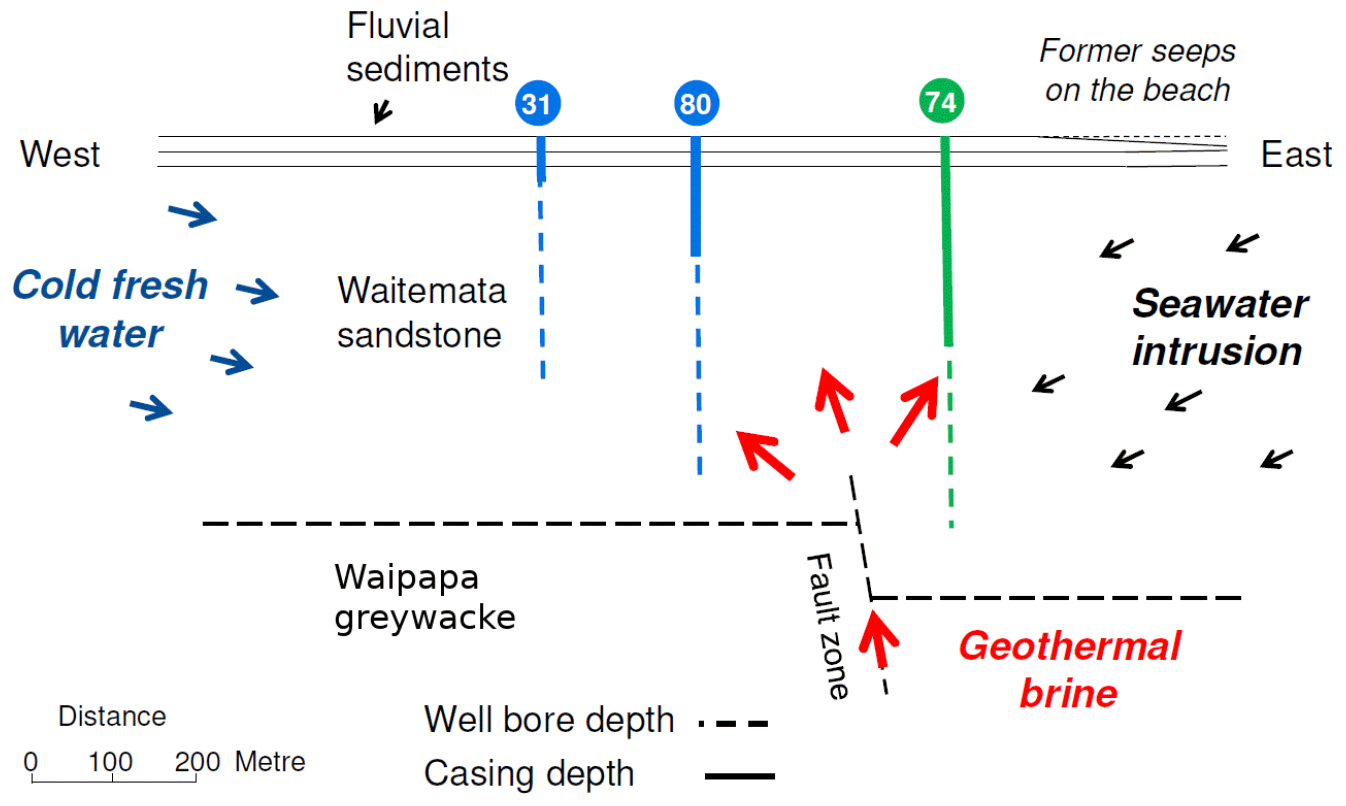
Figure 1 W–E cross section. The arrows depict the flow directions. The bore holes no. 31 and no. 80 are the major production wells (blue colour) and no. 74 is the observation well (green colour) close to the sea (modified after Kühn and Altmannsberger, 2016).

2.2 Production rates and water level data

For the water level data, an hourly and a daily averaged time series from the observation well no. 74 (Fig. 1) were available. The data cover a period of almost 40 years from 1982 to 2019. The data set is not fully continuous and shows gaps ranging from a few days up to several months. Gaps smaller than 3 d in maximum were interpolated linearly.

The water level readings were corrected first for the atmospheric pressure load, because the aquifer is confined. For this purpose, atmospheric pressure data from the two nearest available stations was used (NIWA¹). Station “Whenuapai Aero” is 28.5 km away from the centre of Waiwera and was used to cover the time range from the beginning of the water level measurements in the 1980s until the year 2010. Station “1340” is 31.6 km away and covered the remaining time until today. For each station, a linear regression between daily atmospheric pressure change ΔP_atmo and daily water level change was conducted. The slope of the regression line is the barometric efficiency B which for “Whenuapai Aero” and “1340” was 0.59 and 0.52, respectively. The corrected water level p_cor is then calculated from the actual water level reading p_old and γ the specific weight of water following Eq. (1):

$$\begin{array}{}\text{(1)}& p_{\mathrm{cor}}=p_{\mathrm{old}}-B{\displaystyle \frac{\mathrm{\Delta }{P}_{\mathrm{atmo}}}{\mathit{\gamma }}}\end{array}$$

The production rate data were available as time series for the two main wells, no. 31 and no. 80 (Fig. 1). The data is continuous without any gaps. For the work presented here, the sum of both rates was used. The analysed range of the production data starts December 2005 and ends June 2017. From prior studies it is known that the Kaikoura Earthquake in 2016 induced significant water level changes in the reservoir and maybe even changed its properties (Kühn and Schöne, 2018). Therefore, the analysed time range was further confined to one day before the earthquake (13 November 2016) as the last day.

2.3 Implementation, boot strapping and synthetic data simulation

The implementation of the algorithm strictly follows the description of the variable projection algorithm in the original paper of Von Schroeter et al. (2004). It is the standard algorithm for separable least squares problems and requires the solution of two parts in each iteration. One is based on the mathematical QR decomposition and one on Singular Value Decomposition (SVD). The advantage of the scheme is its applicability for large data sets. In the following we only describe the adaptions we made for the presented study:

• within the variable projection algorithm, both, the linear and non-linear sub-problems are being solved using the singular value decomposition;

• because the rate and the water level data are both given with a daily resolution the total least squares (TLS) system turns out to be underdetermined when incorporating the estimation of true rates. Therefore, only the water level error and the measure of curvature are part of the TLS, not the rate error.

From these two points, the new TLS is deduced via the convolution matrix C, the derivative matrix D, the naturally unaffected water level p₀ and the column vectors γ and k with:

$$\begin{array}{}\text{(2)}& E\left(p_{\mathrm{0}},z\right)={∥{\mathit{p}}_{\mathrm{0}}\mathit{\gamma }-\mathit{p}-\mathbf{C}\left(z\right)\mathit{q}∥}_{\mathrm{2}}^{\mathrm{2}}+{\mathit{\lambda }}^a{∥{\mathbf{D}}_z-\mathit{k}∥}_{\mathrm{2}}^{\mathrm{2}}\end{array}$$

The estimation of the regularisation parameter λ will be specified with an additional, adjustable exponent a. This is done to variate the initial regularisation parameter defined as:

$$\begin{array}{}\text{(3)}& {\mathit{\lambda }}_{\mathrm{def}}={\displaystyle \frac{{∥\mathbf{\Delta }\mathit{p}∥}_{\mathrm{2}}^{\mathrm{2}}}{m}}\end{array}$$

with the number of hydraulic head data points m in such a way that the resulting response curve becomes smooth enough to be interpretable, as mentioned by Von Schroeter et al. (2013). Because smoothness is a subjective criterion, the adjustment of the initial regularisation parameter requires careful investigation. For this, the result has been investigated with different exponent values that range from high (close to zero) to low (greater negativity). For values being too high the response function is stiff and suppresses features while for values being too low it achieves an excessive level of freedom and shows high-frequency features with no physical meaning. The optimal choice of smoothness lies in between and has been identified by a gradual decrement of the exponent a until a response function is generated where the dominant features still exist and are interpretable, but arose from the maximum possible freedom, i.e. the lowest possible exponent.

To increase the reliability of the result and to also derive the statistical values of the response function seen as a dependent random variable, the algorithm was subjected to a bootstrapping method. In each of the 1000 iterations, a fortnightly time period was randomly sampled from the entire time range. Even though the initial regularisation parameter λ_def as well as the initial guess of the response function are estimated individually for each run, the following parameters remained constant and were predefined as follows:

• the first and best guess of the naturally unaffected water level p₀ was the mean water level between January and September 2019 which comes closest to the end of the build-up curve after the main spa in Waiwera closed down;

• the total number of nodes was set to 36; according to Von Schroeter et al. (2004) the number of nodes is arbitrary within the constraints that an increment of nodes will increase the resolution while also putting the TLS problem at a higher risk of being underdetermined; here, the number of 36 nodes ensures a resolution which is still equal to that of one day at the end of a fortnightly period; an underdetermined TLS problem could not be detected even for much higher number of nodes since the adjustment of the exponent a always seemed to compensate for it;

• the first node was set to one day due to the respective resolution of the time series.

To relate true response functions with corresponding functions found by the algorithm, three simulations with synthetic data were conducted. In doing so, the actual physical flow behaviour may be linked to the bootstrapping results from an empirical point of view. This extends the pure mathematical evaluation which, as to be seen later, turns out to be not always feasible. For the three simulations, three different scenarios were assumed.

The first and the second one are referring to radial flow for the first day followed by a Leaky Flow Boundary (LFB) or a Constant Head Boundary (CHB), respectively. We regard these two scenarios as the most likely ones for the reservoir. Their parameterisation is mainly based on the results of the pumping test from 1979 (ARWB, 1980). The only exceptions are the parameterisation of the leakage factor and the distance ratio for the LFB and the CHB respectively. These parameters could of course not be deduced from the pumping test and are therefore parameterized to best fit the results of the bootstrapping results while still lying in a physically reasonable value range. The third scenario represents the assumption of the pumping test itself and assumes an instant steady-state (ISS) condition as expressed by the Thiem solution. The parameters from the pumping test are applied in this case as well.

The explicit formulation for all three scenarios is as follows:

• one day radial flow, followed by a Leaky Flow Boundary (LFB):

  For radial flow the response function to the power of e is:

  $$\begin{array}{}\text{(4)}& {\displaystyle \frac{\partial G}{\partial \ln \left(t\right)}}={\displaystyle \frac{\partial }{\partial \ln \left(t\right)}}\left({\displaystyle \frac{\mathrm{1}}{\mathrm{4}\mathit{\pi }T}}\ln \left({\displaystyle \frac{\mathrm{2.25}Tt}{r^{\mathrm{2}}S}}\right)\right)={\displaystyle \frac{\mathrm{1}}{\mathrm{4}\mathit{\pi }T}}\end{array}$$

  The resistance function G is parameterised with the transmissivity of T=320 m² d⁻¹ determined from the pumping test. For a leaky flow boundary the drawdown is calculated after Walton's method described by Kruseman et al. (1990) under the valid assumption of a negligible aquifer storativity S:

  $$\begin{array}{}\text{(5)}& G\left(u\right)={\displaystyle \frac{\mathrm{1}}{\mathrm{4}\mathit{\pi }T}}\underset{u}{\overset{\mathrm{\infty }}{\int }}{\displaystyle \frac{e^{\left(-u-\frac{r^{\mathrm{2}}}{\mathrm{4}{\mathit{\beta }}^{\mathrm{2}}u}\right)}}{u}}\mathrm{d}u\end{array}$$

  From this equation, the response curve to the power of e can be derived as:

  $$\begin{array}{}\text{(6)}& {\displaystyle \frac{\partial G}{\partial \ln \left(t\right)}}={\displaystyle \frac{\mathrm{1}}{\mathrm{4}\mathit{\pi }T}}{e}^{\left(-u-\frac{r^{\mathrm{2}}}{\mathrm{4}{\mathit{\beta }}^{\mathrm{2}}u}\right)}\end{array}$$

  with $u=\frac{r_{\mathrm{74}}^{\mathrm{2}}S}{\mathrm{4}Tt}$.

  The function is parametrised with the theoretical storativity suggested in the pumping test, $S=\mathrm{2}\times {\mathrm{10}}^{-\mathrm{3}}$. The leakage factor β is arbitrarily set to 200 which translates to a comparably steep gradient in the response function.

• one day radial flow, followed by a Constant Head Boundary (CHB):

  The linear constant head boundary will be described by Stallman's method described by Kruseman et al. (1990):

  $$\begin{array}{}\text{(7)}& G\left(u\right)={\displaystyle \frac{\mathrm{1}}{\mathrm{4}\mathit{\pi }T}}\left(W\left(u\left(t,r_{\mathrm{74}}\right)\right)-W\left(u\left(t,r_{\mathrm{Ratio}}{r}_{\mathrm{74}}\right)\right)\right)\end{array}$$

  with r_Ratio given by the distance to the imaginary well r_im over the distance to the observation well r₇₄:

  $$\begin{array}{}\text{(8)}& r_{\mathrm{Ratio}}={\displaystyle \frac{r_{\mathrm{im}}}{r_{\mathrm{74}}}}\end{array}$$

  The response function to the power of e is then:

  $$\begin{array}{}\text{(9)}& {\displaystyle \frac{\partial G}{\partial \ln \left(t\right)}}={\displaystyle \frac{\mathrm{1}}{\mathrm{4}\mathit{\pi }T}}\left(e^{-u\left(t,r_{\mathrm{74}}\right)}-e^{-u\left(t,r_{\mathrm{Ratio}}{r}_{\mathrm{74}}\right)}\right)\end{array}$$

• Instant Steady State (ISS) case within the first day, as inferred from the pumping test:

  here the response function to the power of e is a Dirac delta function scaled by the same factor as the Thiem equation used for pumping tests

  $$\begin{array}{}\text{(10)}& {\displaystyle \frac{\partial G}{\partial \ln \left(t\right)}}=\mathit{\delta }\left({\displaystyle \frac{\log \left(r_{\mathrm{74}}\right)\mathrm{2}\mathit{\pi }tT}{\log \left(r_{\mathrm{nat}}\right)\mathrm{2.3}}}\right)\end{array}$$

  The function is parametrised with the transmissivity from the pumping test. Further, r₇₄ is the distance between the observation well no. 74 and the production wells which is estimated with 140 m. r_nat is the distance to a position where the water level is assumed to be unaffected by water production. From the drawdown distribution during the pumping test the distance was estimated to be 240 m.

The overall creation of synthetic data works as follows:

• the true response function is defined based on each scenario of the flow behaviour to be simulated;

• random production rates are created following a normal distribution with the same first and second moments like the measured rates;

• the water level is calculated by conducting a forward convolution;

• the production rate data are perturbed with a given error level. This error level corresponds to 10 % of the standard deviation of the measured production rate data. Compared to other error levels this is a quite high estimate.

The production rate data and the water level are then fed into the algorithm and the resulting response function can be compared with the true response function (Grabow and Kühn, 2021).

3 Results of the well test analysis

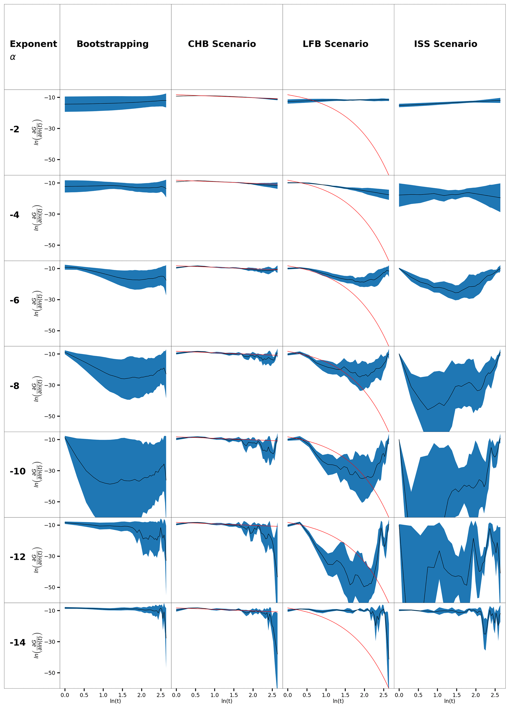
The results of the bootstrapping algorithm and the three synthetic data simulations are shown in the corresponding columns of Fig. 2. Each row refers to a different exponent a. In each plot the y axis has the unit of the response function while the x axis displays the nodes.

Owing to the occurrence of outliers the representative response curve is derived from the median of all response curves and is shown in black. For the same reason, the median absolute deviation (MAD) of all response curves is used as the representative quantity of statistical dispersion. It is depicted as a blue area which expands below and above the median response function for a given MAD value. Further, for the LFB and CHB scenarios the true response curve is shown in red.

For the evaluation and the subsequent discussion name conventions of early, middle and late times in accordance with Gringarten (1985) are used. Whereas early times belong to characteristic flow close to the well and is not considered in this study, middle times will be equivalent to the processes during the first day. Anything later where flow boundaries become present are called for as late times.

3.1 Response functions

For the bootstrapping with exponents of $a=-\mathrm{2}$ to $a=-\mathrm{4}$, the median curve is almost horizontal and with values for the first node of −14.4 up to −12.3, respectively. For lower exponents down to $a=-\mathrm{10}$ the curves develop a characteristic shape with a sharp decline at the beginning and a linear increases towards the end. At the very end, we observe again a sharp drop.

For the exponent of −10 this shape leads to a global minimum at times of roughly $t=e^{\mathrm{0.5}}=\mathrm{1.6}$ d and to a less distinct local maximum at times of $t=e^{\mathrm{2.5}}=\mathrm{12.2}$ d. The intersection with the y axis rises with the evolution of the shape with decreasing exponents. For the exponent of −10 the first node has a value of −8.7. For even smaller exponents the shape reverses and the depression slowly disappears until the curve is almost horizontal again. However, the sharp drop at the end remains accompanied by increasingly large, high-frequency fluctuations that superpose the overall shape for later times.

The MAD remains relatively small and constant throughout the whole time for the application of larger exponents. With the development of the mentioned characteristic shape with $a=-\mathrm{4}$ and below it clearly increases for across the entire investigated time frame, except for the very first node where it remains small irrespective of the applied exponent. For exponents smaller than $a=-\mathrm{12}$ the MAD decreases again, except for very late times where the fluctuations of the median response curve are observed.

Figure 2 Results of the bootstrapping algorithm and the three synthetic data simulations.

3.2 Synthetic data simulation

For the CHB scenario the median response curve shows the best fit compared to the true response function with high exponents already for $a=-\mathrm{2}$. With decreasing exponents, the median response starts deviating especially for later times while at the beginning it remains almost unchanged. The deviation mainly originates from the fluctuations. It is observed as well that the MAD increases with decreasing exponents, especially towards the late times where the fluctuations occur.

For the LFB scenario the median response function starts again with a horizontal line which aligns more and more to the true response function between the start and roughly $t=e^{\mathrm{1.5}}=\mathrm{4.5}$ d with decreasing exponents from −4 to −8. The values for very late times remain almost constant which leads to an upward trend after 4.5 d and the development of a global minimum. Notably, the value of the first node is always underestimated by the algorithm. With smaller exponents down to $a=-\mathrm{12}$ the global minimum decreases further and at the same time the curves experience larger fluctuations which start comparatively early. With even lower exponents the median response function changes its shape and develops back to a horizontal line with fluctuations at the end. The MAD generally increases with decreasing exponents down to $a=-\mathrm{12}$. This is especially observed during the middle period, whereas for very late times the increase is only little. For early times however, it remains more or less constant. When the median response function becomes a horizontal line again along the x axis of ln(t), the MAD decreases significantly and only increases for very late times when fluctuations are present.

The median response function of the ISS scenario shows a similar development as the one of the LFB scenario with decreasing exponents. That is, the curve is an almost horizontal line for higher exponents and then develops more and more a minimum down to $a=-\mathrm{6}$. With even lower exponents down to $a=-\mathrm{12}$ this global minimum becomes more pronounced and its position moves further towards earlier times. This is accompanied by a strong increase of the fluctuations at later times. With exponents smaller than −12, the curves turn into horizontal lines again with fluctuations similar to the ones for the CHB and LFB scenarios. The MAD is generally quite high except for very high and very small exponents. In all cases it is high right from the start until later times for high exponents down to $a=-\mathrm{12}$. Like for the two other scenarios the MAD decreases slightly for very late times. For exponents below $a=-\mathrm{12}$ the MAD decreases in general but remains high for the late times where the fluctuations are observed.

4 Discussion

4.1 Mathematical evaluation

We do see the exponent of −10 as most suitable for further interpretation of the response functions for the investigated system. This is due to three reasons. First, it satisfies the requirement, coming from higher exponents, to correspond to the lowest regularisation parameter which yields a response function that is still interpretable and as well features the shape that is seen as valid. A valid shape is considered to be the development of the global minimum, just by exclusion of the other two shapes, i.e. the almost horizontal lines for very high and low exponents. In comparison with the simulated scenarios these are regarded as shapes of artificial origin. Second, it corresponds to one of the lowest regularisation parameter, which still ensures a stable parameterisation of the algorithm for which 998 out of 1000 samples yielded a solution. Third, among these first regularisation parameters, it yields a response function with the lowest MAD at the beginning of the curve. Because only the evaluation of middle times allows the comparison with the results from the pumping test, low variability at the beginning is especially desirable.

So far only the mathematical evaluation of middle times is thought to be meaningful. For later times, after one day, the MAD becomes too high to regard the median response curve as a representative outcome. For this reason, only the first node will be evaluated which also means that, in contrast to usual well test evaluations, the flow behaviour cannot be inferred from the shape of the response function. Only the value of the first node itself may give an indication for it. So far, only the assumption of radial flow during the first day led to a transmissivity value, which also comes close to the findings of the pumping test:

$$\begin{array}{}\text{(11)}& {\mathit{\tau }}_{\mathrm{1}}=\ln \left({\displaystyle \frac{\mathrm{1}}{\mathrm{4}\mathit{\pi }T}}\right)\end{array}$$

With the node ${\mathit{\tau }}_{\mathrm{1}}=-\mathrm{8.69}$ the transmissivity equates to roughly 474 m² d⁻¹. A MAD of 0.99 translates into an asymmetric confidence interval for T with T=1281 m² d⁻¹ as the upper boundary and T=176 m² d⁻¹ as the lower boundary.

4.2 Comparison with simulated data cases

For high exponents, the algorithm yields an almost horizontal curve for all three scenarios (Fig. 2). This is reasonable because the initial guess of the function is a horizontal line and the regularisation parameter at this stage is high. Therefore, any deviation from the initial curve, which inevitably disturbs smoothness, i.e. increases the second derivative, is penalised to a great fraction in the objective function. The optimum is then found close to that of a horizontal line. The fact that the true response function of the CHB scenario is estimated quite well may therefore be explained by its smaller negative slope which comes closer to a horizontal line than the true response curve of the LFB. Even though the shape of the LFB and the ISS scenario cannot be estimated at this stage, the value of the first node which corresponds to middle times is estimated well for all three scenarios. For the results of the bootstrapping method this means that the middle time behaviour may also be regarded as valid.

The phenomenon that for very low exponents again a horizontal line happens to be the median response curve for all three scenarios can be explained by the considerably lower number of successful samples. On the one hand, this translates into less curves that can be considered for evaluation which decreases the MAD. On the other hand, it creates a bias of the solution spectrum since the curves from a successful run satisfy certain properties. The reason why a solution cannot be found is not because the algorithm did not converge but rather because the response functions achieved values that are too low to be computationally handled. Since in addition fewer solutions are found right above these limiting values the median depicts the left-over majority of curves which are solutions of the horizontal line close to the initial guess.

Considering the development of the median response function over the course of decreasing exponents for the LFB scenario, it seems that the good fit until day 4.5 for $a=-\mathrm{6}$ is purely accidental. Beside the good fit for middle times the curve goes down arbitrarily and up again with a high value of the MAD and therefore a broad spectrum of other solutions being completely different than represented by the median curve.

A similar arbitrary development can be seen for the ISS scenario after the first day. Because here a mathematical relation between water level and rate data does not exist after the first day, fluctuations as well as the high MAD must be regarded as the algorithms behaviour to such circumstances. Therefore, the fluctuation as well as the MAD in the LFB scenario may also be dedicated to a lack of obvious connection between water level and production rate data. This can be the case because the true response curve for the LFB reaches down to particularly low values after a short time and a decrease of a response function value equates to an exponential decrease of the function the rate series is convoluted with. In other words, even though mathematically the influence of production rates still exists, below some value, the superposed rate error overweighs this influence and no serious relation can be found by the algorithm. Because the results of the bootstrapping method show a similar large MAD it is then likely that the true response function of the reservoir also reaches down to very low values. This leads to the assumption that either a LFB with a comparable low leakage factor or an instant equilibrium like in the ISS scenario is present. Considering the history of the reservoir during which an excessive exploitation led to a steady decline over decades as well as the build-up curve which extended over nearly two years, the latter is regarded as unrealistic. With the mathematical findings for middle times, a radial flow behaviour within the first day followed by a leaky flow behaviour for later times is seen as the most plausible result based on the current findings.

4.3 Errors and uncertainties

The biggest source of error comes with the assumption that bore holes no. 31 and no. 80 are the only production wells. In contrast, a lot of other bores exist (Kühn and Stöfen, 2005) from which also water is produced on a regular basis. This fact must be accepted owing to the lack of other data.

Another error might arise from taking the sum of both rates and so to treat the system with effectively only one bore. However, the error likely affects only the early-time behaviour which cannot be seen on a daily resolution. To account for both wells individually the program should be extended to a multi-well deconvolution problem like it has been done by Cumming et al. (2014). For now, the error due to summation is still lower than the error which would result from selecting only one well and neglecting the other.

Furthermore, apart from the barometric effect, other influences on the hydraulic head were neglected. It must be acknowledged that the hydraulic head values which were used in this analysis do not relate to production rates only. Other effects might be the loading of the overlying fresh water aquifer, variation in groundwater recharge and varying boundary conditions, especially the tides on the sea side.

A conceptual error arises from deconvolution itself which implies a linear system with the principle of superposition in time. For larger fractures, this condition is often not met according to Kruseman et al. (1990). However, based on the high density of fractures this case might be excluded. Observations from the pumping test showed a spatially homogeneous response during pumping and thus support this assumption.

All these different errors end up in a perturbation that makes it difficult for the algorithm to distinguish it from actual convolution. This can especially be seen for later times where the response function is low and thereby its contribution to water level changes. With the method applied in this work, the uncertainties are too high to allow anything else than to speculate for a type of boundary condition, not to mention its parametrisation.

5 Conclusions

We conclude that the current implementation of a variable-rate well test analysis is applicable to the daily-averaged time series in Waiwera. This is true for middle-time behaviour for which well test analysis yields the same model parameter as the pumping test. The result for late-time behaviour, however, can only be interpreted based on comparison with synthetic data. The outcome indicates very low values for the true response function right after the first day. Considering an instant equilibrium of the reservoir as incompatible with the observations over the past, only a leaky flow boundary with a low leakage factor can be seen as appropriate. It needs to be taken into account that the original method we adapted in the present study was developed for the interpretation of standard well tests. For such set-ups, it is a very powerful tool and is applicable to many hydrogeological settings. However, in situations in which reservoirs react to changing constraints the deconvolution reaches its limits. For the “long term pumping test with varying rates” we tested here, further development is required.

For the future, a more extensive investigation of different flow conditions under different parametrisations should be conducted. Only in this way the statistical dispersion of the outcome could be linked quantitatively to response functions. To also improve data quality, the influence of other environmental factors on the water level should be investigated more extensively. Especially the influence of precipitation and the tides require more analysis.

To overcome the inherent limitation of the deconvolution algorithm implemented here, spectral methods could be tested. This completely different approach would solve the deconvolution in the Laplace/Fourier space and therefore simplify the problem to a pointwise product between two functions.

Appendix A: List of symbols and nomenclature

In order to avoid conversion factors in equations, all quantities appearing in them are assumed to be either dimensionless or to have matching units.

a	adjustable exponent [–]
B	barometric efficiency [–]
C	convolution matrix
CHB	constant head boundary
D	discretized derivative matrix
G	resistance function
γ	column vector with $\mathit{\gamma }=(\mathrm{1},\mathrm{1},\mathrm{\dots },\mathrm{1})\in R^m$
λdef	initial regularisation parameter [–]
ISS	instant steady state
k	column vector with $\mathit{k}=(\mathrm{1},\mathrm{0},\mathrm{\dots },\mathrm{0})\in R^m$
LFB	leaky flow boundary
m	number of hydraulic head data points
MAD	median absolute deviation
p0	naturally unaffected water level [m]
pcor	corrected water level data [m]
pold	water level reading [m]
Patmo	atmospheric pressure [Pa]
rim	distance to the imaginary well [m]
rnat	distance to a position where the water level is assumed to be unaffected [m]
r74	distance to the observation well no. 74 [m]
rRatio	distance ratio [–]
SVD	Singular Value Decomposition
S	Storativity [–]
t	time [d]
γ	specific weight of water [N m−3]
T	transmissivity [m2 d−1]
τn	nth node