 | 26 Feb 2021
Unconstrained Estimation of VLBI Global Observing System Station Coordinates
Markus Mikschi
Johannes Böhm
Matthias Schartner
The International VLBI Service for Geodesy and Astrometry (IVS) is currently setting up a network of smaller and thus faster radio telescopes observing at broader bandwidths for improved determination of geodetic parameters. However, this new VLBI Global Observing System (VGOS) network is not yet strongly linked to the legacy S/X network and the International Terrestrial Reference Frame (ITRF) as only station WESTFORD has ITRF2014 coordinates. In this work, we calculated VGOS station coordinates based on publicly available VGOS sessions until the end of 2019 while defining the geodetic datum by fixing the Earth orientation parameters and the coordinates of the WESTFORD station in an unconstrained adjustment. This set of new coordinates allows the determination of geodetic parameters from the analysis of VGOS sessions, which would otherwise not be possible. As it is the concept of VGOS to use smaller, faster slewing antennas in order to increase the number of observations, shorter estimation intervals for the zenith wet delays and the tropospheric gradients along with different relative constraints were tested and the best performing parametrization, judged by the baseline length repeatability, was used for the estimation of the VGOS station coordinates.
- Article
(2599 KB) - Full-text XML
- BibTeX
- EndNote


In order to improve the accuracies of geodetic parameters determined with Very Long Baseline Interferometry (VLBI) observations, the International VLBI Service for Geodesy and Astrometry (IVS) (Nothnagel et al., 2017) has developed the VLBI Global Observing System (VGOS) (Petrachenko et al., 2009). This new system is based on smaller and faster VLBI radio telescopes, allowing for a significantly increased number of observations, thereby enabling an improved estimation of tropospheric parameters which are considered one of the major error sources in geodetic VLBI (Schuh and Böhm, 2013). A recent demonstration of the possibilities with VGOS based on a single baseline between WESTFORD (USA) and the station GGAO12M (USA) is provided by Niell et al. (2018).
With the number of publicly available VGOS sessions rising, accurate station coordinates for the participating stations become more important, e.g. for the estimation of Earth Orientation Parameters (EOP) in general or the estimation of UT1-UTC from VGOS Intensive sessions in particular. Furthermore, it is necessary to properly connect the VGOS network with the International Terrestrial Reference Frame (ITRF). This enables the combination and comparison of VLBI analysis results from S/X and VGOS sessions which is critical for the further development and testing of VGOS. Thus, this work aims to provide accurate VGOS station coordinates. The main challenge is caused by the fact that the datum has to be defined without accurate a priori coordinates of most stations.
In Sects. 2, 3 and 4, we describe the existing VGOS data set, our methodology of calculating station coordinates, and the results, respectively. Additionally, we investigate the optimal parametrization of tropospheric parameters in Sect. 4.1, which might be different for VGOS sessions compared to S/X sessions.
1.1 Definition of the Geodetic Datum
Normally, at least three stations participating in a session need accurate a priori coordinates in the target terrestrial reference frame for the definition of the geodetic datum. These stations should be globally well distributed and a higher number of stations is beneficial for making the datum definition redundant. Since so far, no VGOS observations have been used in calculating a solution of the ITRF, it is difficult to proceed with standard approaches relying on No-Net-Translation (NNT) and No-Net-Rotation (NNR) conditions on a priori ITRF coordinates of at least three stations. Among the VGOS telescopes, only WESTFORD is listed in the ITRF2014 (Altamimi et al., 2016) based on earlier S/X observations with this telescope. Between 2011 and 2014, WESTFORD was converted to a VGOS station by a receiver change (Niell et al., 2018). While the ITRF2014 coordinates of WESTFORD are derived from the S/X observations, we can safely assume that the coordinates are the same for VGOS observations since the coordinates refer to the intersection point of the axes and are not related to the receiver (Nothnagel, 2018).
The VLBI observations themselves define the relative position of the stations w.r.t each other, the inner network geometry, but not their absolute position and orientation with respect to a specific reference frame. This results in a singular equation system during the least squares adjustment because the design matrix and subsequently the normal equation matrix have a rank deficiency corresponding to the degrees of freedom (DOF) of the network. In the case of VLBI analysis, the DOF is six, where three degrees are related to the rotation and the remaining three are related to the translation of the network. There is no scale ambiguity because the scale is defined directly by the VLBI observations. The definition of the geodetic datum solves that rank deficiency, also called a datum deficiency, and embeds the network geometry in a reference frame.
In the VLBI analysis the least squares approach is used to estimate the most likely values of selected parameters x based on a linearized over-determined equation system with observations affected by random errors. If the individual observations can be expressed solely as a function of the parameters that are estimated, as is the case with VLBI observations, the general case of the least squares approach can be simplified using the Gauss-Markov model (Niemeier, 2008). Thereby, the corrections for the a priori parameters dx can be estimated using
with A being the Jacobian matrix containing the partial derivatives of the functional model w.r.t the estimated parameters and AT the transposed matrix, P denoting the weight matrix for the observations and l the vector “observed” minus “computed with a priori values”. N is called the normal equation matrix and is computed using ATPA. In the presence of a datum deficiency the matrix is singular and thus Eq. (1) cannot be solved.
There are two methods of defining the geodetic datum in a least squares adjustment for the VLBI analysis without affecting the inner network geometry:
-
Free Adjustment. This is the most commonly used datum definition method during the analysis of geodetic VLBI sessions. In this method, also known as the minimal constraint method, carefully selected reference stations with very accurate a priori coordinates (x, y, z) are selected as the datum stations. Their a priori coordinates are used together with the estimated additions to the a priori coordinates (dx, dy, dz) to form the NNT/NNR conditions. The NNT conditions stipulate that the sum of the estimated additions to the a priori coordinates of the datum stations along all three axes has to be zero. Similarly, the NNR conditions ensure that the sum of rotations about all three axes is zero.
The NNT and NNR conditions are represented as the matrix-vector multiplication Gdx=0. Subsequently the N matrix is extended by G. The extended matrix is now regular and the equation system can be solved. Therefore, Eq. (1) becomes Eq. (2).
The benefit of this method is that the coordinates of the datum defining stations are still estimated and their accuracy can be calculated. Furthermore, the datum can be defined redundantly by selecting more datum stations than the minimum number of three, placing less emphasis on any individual station and potential errors in its a priori coordinates. Because of this and the fact that a good global distribution of the selected stations improves the datum definition, most of the time more than three stations are used in VLBI analysis.
-
Unconstrained Adjustment. In this method the datum deficiency is alleviated by not estimating certain parameters and therefore fixing them to their a priori values. Just enough parameters are fixed such that the datum deficiency is resolved but no constraints or distortions are introduced to the inner network geometry. The parameters are fixed by removing the corresponding columns of the Jacobian matrix A or equivalently removing the corresponding columns and rows of the normal equation matrix N. The benefit of this method is that fewer and potentially more precise a priori values can be used to define the geodetic datum with a potential improvement in the estimated parameter accuracy. A drawback of this method is that the fixed parameters are not estimated and their a priori values are considered as the true values. Furthermore, the datum definition cannot be made redundant since fixing more parameters than necessary imposes a constraint on the inner network geometry which would potentially contradict the observations. An adjustment in which more parameters than necessary are fixed to their a priori values is called an constrained adjustment. However, it has no relevance for the task described here.
1.2 Tropospheric delay parametrization
Tropospheric delays are generally modelled as the delay in zenith direction related to the delay at any given observation elevation angle by a mapping function (Nilsson et al., 2013). In this study, we use the Vienna Mapping Functions 3 (Landskron and Böhm, 2018). The modelled delay is divided into a hydrostatic and a wet delay. While the hydrostatic zenith delay can be determined from pressure measurements at the stations (see Saastamoinen, 1972 and Davis et al., 1985), the modelling of the wet delay is more difficult. Thus, zenith wet delays (ZWD) are estimated in the VLBI analysis. To account for azimuthal asymmetries in the tropospheric delays, so-called horizontal tropospheric gradients are also estimated. The ZWD and gradients are varying phenomena and as such have to be parametrized in a way that allows for temporal variability while keeping the number of estimated parameters low in order to maintain an over-determined equation system. This can be achieved by using piecewise linear offsets (PWLO) for the parametrization of the ZWD and gradients (Schuh and Böhm, 2013). PWLO are based on offsets at certain reference epochs and linear interpolation in between. Typically used estimation interval lengths are 30 min for the ZWD and 180 min for the gradients. Those values are used by the Vienna VLBI analysis center as of the time of writing. Additionally, relative constraints between the offsets can be introduced to increase numerical stability and avoid singularity issues caused by too few observations during any given estimation interval. The constraints are realized as pseudo-observations, stipulating that the parameter at epoch ti+1 has to be equal to the parameter at ti. The strength of the constraint is set by the associated accuracy of the pseudo-observation during the least squares adjustment.
For this study 30 VGOS sessions from 2017 and 2019 were used. Five sessions in 2017 were observed as part of the CONT17 campaign (see https://ivscc.gsfc.nasa.gov/program/cont17/, last access: 24 February 2021) and therefore are concentrated in December 2017. The remaining 25 are distributed over 2019. All sessions lasted for 24 h and the names of the sessions along with the participating stations can be seen in Fig. 1. The CONT17 sessions started at 23:00 UTC while the sessions in 2019 started at 18:00 UTC.

Figure 1Station activity during the VGOS sessions used in this study. The first five sessions were part of the CONT17 campaign. ISHIOKA does only have VGOS observations during CONT17 and at the end of 2019. In between, it participated in S/X sessions.
Potential effects of the cluster of CONT17 sessions were investigated. The difference in the estimated coordinates, when the five CONT17 sessions are excluded, is below 1.5 mm for all stations except for ISHIOKA and the z-coordinate of KOKEE12M. The larger differences for ISHIOKA are to be expected since five of seven sessions in which ISHIOKA participated are in 2017. As ISHIOKA is the closest station to KOKEE12M, its coordinates are also influenced by this. Since no velocities are estimated from the VGOS data in our study, the CONT17 sessions should not act as leverage observations and therefore should not skew the estimated parameters in a significant way. It was opted to include the CONT17 sessions for an increase in observations.
Figure 2 depicts the resulting station network. In general, VLBI suffers from an imbalance of station distribution since there are far more stations in the northern than in the southern hemisphere (Plank et al., 2015). This imbalance is even more pronounced for the VGOS station network, as all stations available for this study are in the northern hemisphere with concentrations in Europe and the East Coast of the USA. However, since the aim of this study was to estimate station coordinates within an existing TRF and not to estimate a TRF there should not be strong effects of this imbalance. The fact that most stations are rather close to WESTFORD should in fact benefit the accuracy of the estimated coordinates because of the used datum definition (see Sect. 3.1).

Figure 2The VGOS station network used in this study. All stations are located in the northern hemisphere. Onsala (Sweden) runs a twin VGOS telescope with a north-east (ONSA13NE) and a south-west (ONSA13SW) dish.
All analyses were carried out with the Vienna VLBI and Satellite Software (VieVs) (Böhm et al., 2018) following the Conventions 2010 of the International Earth Rotation and Reference Systems Service (IERS) (Petit and Luzum, 2010) and their updates.
3.1 Station coordinate estimation
First, we ran single session analyses in order to detect and remove session anomalies, such as clock breaks. This preparatory step is characterized by an iterative determination of approximate station coordinates, which allows the detection of problems within the sessions and the continuation with the next steps.
Subsequently a first global solution was calculated by solving all sessions together in a multi-year solution. The global solution uses a combination of the datum free normal equation matrices of the single session analysis to estimate parameters with higher accuracy (Schuh and Böhm, 2013). The geodetic datum for the global solution was defined in an unconstrained adjustment by fixing some parameters to their a priori values, as described in Sect. 1.1. There are multiple possible combinations of fixed parameters that can alleviate the datum deficiency. In this study, the coordinates of the station WESTFORD were fixed to the ITRF2014 solution and the EOP were fixed to the IERS14 C04 (Bizouard et al., 2019) time series in an unconstrained adjustment. Since the EOP describe the transformation between the terrestrial reference frame (TRF) and the celestial reference frame (CRF), fixing them results in the TRF being tied to the CRF. Therefore, the three DOF describing the rotation of the TRF are accounted for by the datum definition of the CRF. Fixing the coordinates of the station WESTFORD addresses the remaining three DOF of the translation of the network. Station WESTFORD was selected for this purpose since it is the only VGOS station with ITRF2014 coordinates. The positions of the radio sources were fixed to their coordinates in ICRF3 (Charlot et al., 2020).
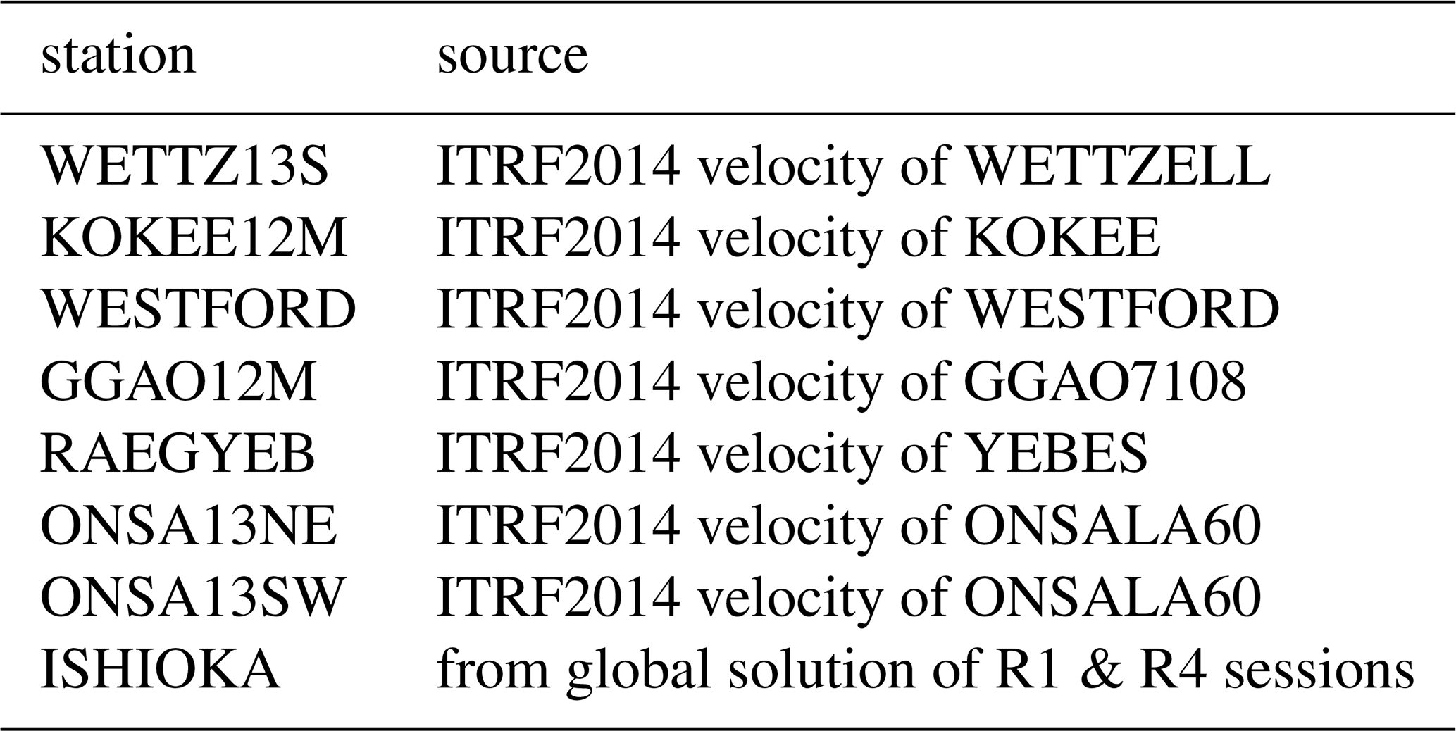
Due to the limited time span of the VGOS data, the station velocities were not estimated during the global solution, but instead fixed to velocities from co-located ITRF2014 S/X stations. It was assumed that the velocities of the nearby S/X stations are identical with the velocities of the VGOS stations. This is a reasonable approach since the S/X station velocities are known with a higher accuracy compared to what would be achievable from the short VGOS time span. However, one exception refers to station ISHIOKA (Japan) as ISHIOKA's velocities could not be fixed to the closest ITRF2014 defining station, TSUKUB32. During tests with velocity estimation in the global solution, the estimated velocity of ISHIOKA was vastly different from the one listed in the ITRF2014 for TSUKUB32. To overcome this discrepancy, the velocity of ISHIOKA was calculated using an independent global solution of 305 R1 and R4 (S/X) sessions from 2017–2019 most of which ISHIOKA participated in. The inconsistencies between the TSUKUB32 and the ISHIOKA station velocity might be explained by the strong tectonic activity in Japan. Table 1 summarizes the sources for the station velocities.
Table 1Sources of station velocities. The velocity for all but one station was taken from corresponding S/X stations except for ISHIOKA, where the velocity was derived from R1 and R4 sessions.
3.2 Troposphere parametrization test
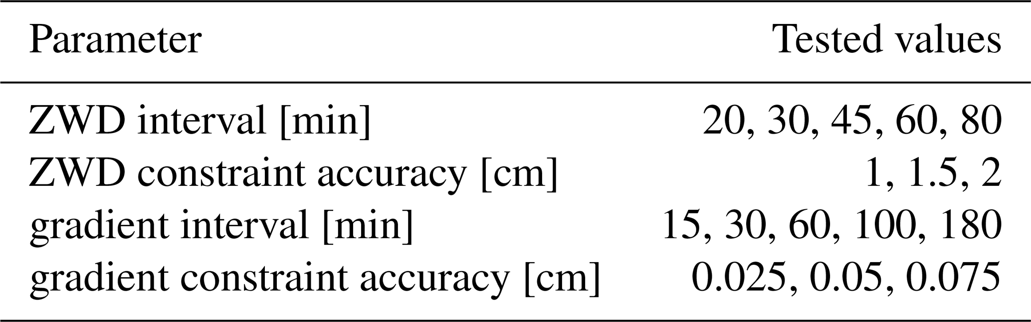
In order to investigate the effects of different troposphere parametrizations on the VGOS sessions, the single session analysis was performed repeatedly, using a grid-wise combination of various ZWD and gradient estimation intervals as well as different constraint accuracies for both parameters. This leads to a four-dimensional parameter space that is investigated. Similarly to the global solution, the datum definition of this single session analysis for the troposhpere analysis was performed by fixing the EOP and the WESTFORD station coordinates. Therefore, three sessions had to be excluded since WESTFORD did not participate (see Fig. 1). The tested values for the different parameters are listed in Table 2. In total, these values lead to 225 different parametrizations.
Table 2Tested values of the parametrization of the tropospheric estimates.
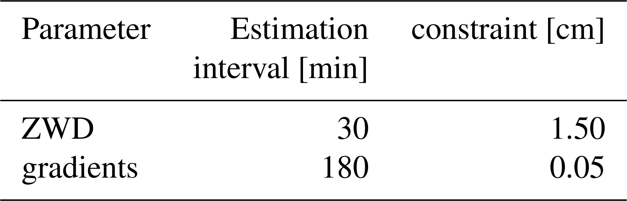
The performance of individual parametrizations was assessed based on the average relative improvement of the baseline length repeatability (BLR) compared to a reference solution. For a specific parametrization the BLR of all baselines was calculated and then individually compared to the corresponding BLR from the reference solution. The relative improvement of all BLRs for one parametrization was averaged to obtain the final metric. The reference solution was derived by selecting a tropospheric parametrization that is typically used for analyzing S/X observations (see Table 3). By investigating the relative improvement of the BLR compared to a reference solution instead of a mean BLR, the dependency on the baseline length can be taken into account, as longer baselines tend to have a worse BLR.
Table 3Parametrization of the tropospheric estimates for the reference solution.
After the best performing troposphere parametrization had been found, the global solution was calculated again as described previously using the improved troposphere parametrization to estimate the final station coordinates with highest precision.
In this section we first investigate the optimal tropospheric parametrization for the VGOS sessions. Then, we present the VGOS station coordinate estimates resulting from the unconstrained adjustment utilizing the best tropospheric parametrization as described in Sect. 3.
4.1 Troposphere parametrization
Table 4 lists the ten best performing parametrizations out of the 225 tested setups, along with the resulting average BLR improvement. As can be seen, best results can be achieved by using shorter estimation intervals for the gradients combined with slightly longer estimation intervals for the ZWD compared to the reference parametrization that is typically used for S/X observations. The six best parameter sets all utilize the combination of 15 and 45 min estimation intervals for the gradients and the ZWD, respectively, with various combinations of the associated constraints.
Table 4The ten best performing troposphere parametrizations out of the 225 tested parametrizations along with the resulting average BLR improvement.

Figure 3 depicts a two-dimensional slice from the four-dimensional parameter space along the interval axes. Since the constraints do not affect the solution that much, this enables to easier compare the improvement based on the different intervals. The importance of short gradient estimation intervals is emphasized as a 15 min interval yields the best results. One exception refers to a ZWD interval of 60 min where longer gradient intervals lead to a better result. The reason for this behaviour is unknown and subject to further investigation.
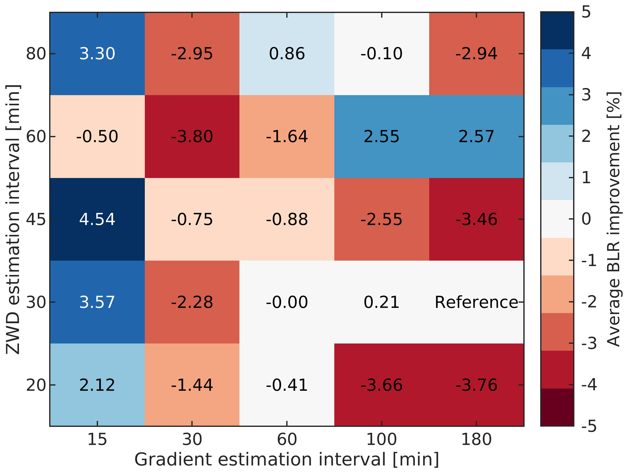
Figure 3The average relative BLR change for a two-dimensional slice from the four-dimensional parameter space along the interval axes for constraints with 1.5 and 0.05 cm for the ZWD and gradients respectively. Blue color denotes improvement, red color degradation.
The selection of the ZWD constraints appears to have a smaller impact on the result. This could be somehow expected since all three constraint values are rather loose and only help to stabilize the solution in case of missing observations between estimation epochs. As far as the gradient constraints are concerned, the highest value (loosest constraint) is yielding the best BLR. This again confirms the importance of rapid and flexible gradient estimates with VGOS, as tighter constraints would eliminate some of the freedom in the estimation gained by the short estimation intervals. However, also for the tightest tested constraints, the combination of 15 and 45 min estimation intervals for the gradients and ZWD, respectively, yields the best results.
The average BLR improvement suggests that shorter intervals do in fact benefit the modeling of real troposphere variations and not just absorb measurement noise. Furthermore, significant changes in the tropospheric delays at low elevations may occur more often, making the rapid gradient estimation more beneficial than the rapid estimation of ZWD. This also holds true for S/X observations and an optimization of the parametrization of these sessions might also be warranted. However, the lower number of observations and the reduced sky-coverage of S/X observations make rapid troposphere parameter estimation difficult. The smaller, faster slewing VGOS antennas enable more observations and a better sky-coverage. Figure 4 shows the number of observations per hour for the different VGOS stations along with the data for all stations of the R1 and R4 sessions during 2019 for comparison. The plot is based on the scheduling files (.skd) of the sessions.
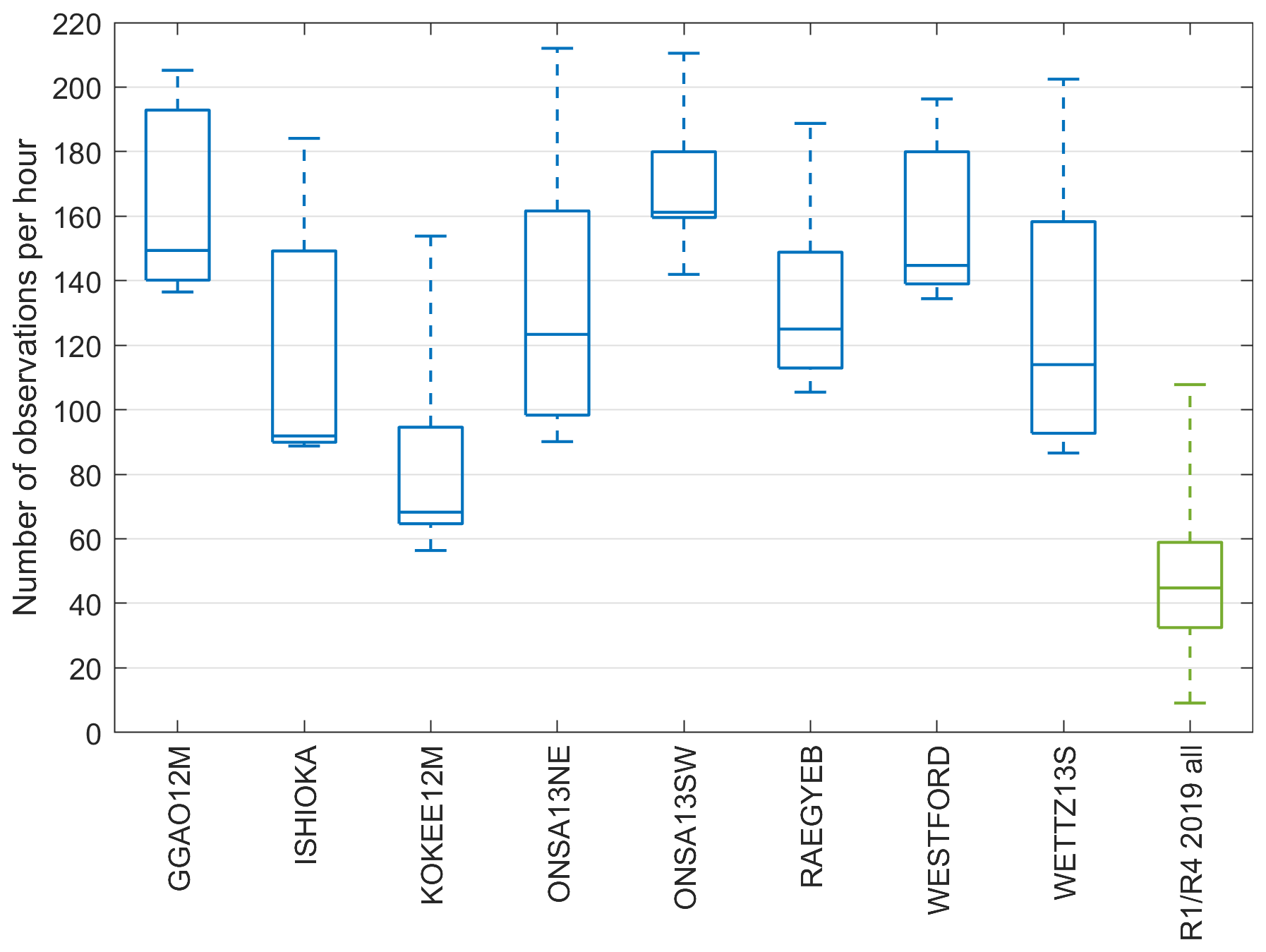
Figure 4Number of observations per hour for the VGOS stations as boxplots. Boxplot for all stations for the R1 and R4 sessions of 2019 added for comparison.
The DOF of a least squares adjustment utilizing such a parametrization is of course lower when compared to the reference parametrization. However, the used VGOS sessions of 2019 still have an average DoF of 5411 or an average ratio between observations and parameters of about 4.8. Therefore we think it is worth the trade-off. Additionally, the introduced relative constraints minimize adverse effects of the shorter estimation interval.
Although sophisticated simulations (Petrachenko et al., 2009) already indicated that rapid gradients will be beneficial for VGOS analysis, this is the first time to see this effect with real data. It is expected that the improvement will even be more visible with further optimized VGOS schedules (Schartner and Böhm, 2020).
The BLR with the reference parametrization that is usually used in the analysis of S/X observations (Table 3) along with the BLR with the best parametrization found within this study is visualized in Fig. 5. It is evident that improvements were achieved for almost all baselines with the two notable exceptions being ISHIOKA–KOKEE12M and KOKEE12M–ONSA13NE. The degradation of the BLR for those two baselines can be explained by the lower number of observations per time for the station KOKEE12M, as can be seen in Fig. 4. The reason for the lower number of observations is the network geometry as KOKEE12M is quite secluded from the rest of the network (see Fig. 2). This problem is expected to be solved by the growth of the VGOS network, as well as improved SNR based scheduling approaches which should yield more observations overall.
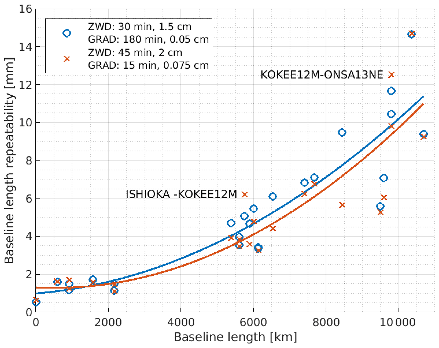
Figure 5Baseline length repeatability of the reference parametrization (blue) and the best parametrization (red) with a fitted second degree polynomial approximation.
Consequently, this parametrization defined in the first row of Table 4 is used for the determination of the VGOS station coordinates. The difference of the estimated station coordinates in the global solution between the best and the reference parametrization is depicted in Fig. 6 in the local east, north, and up components. The European stations exhibit similar shifts while the difference of coordinate estimates for GGAO12M is very small, presumably due to the close proximity to WESTFORD, which was fixed to its a priori values. ISHIOKA and KOKEE12M also exhibit larger changes in the north component. This can be explained by the sky-coverage at those stations, as the observations are limited to one side of the sky due to the network configuration.
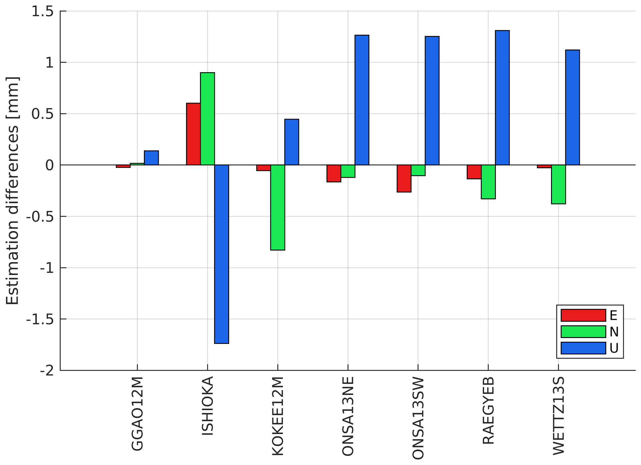
Figure 6Difference in station coordinate estimates from a global solution between the best and the reference troposphere parametrization in the local east, north, and up components.
4.2 VGOS station coordinates
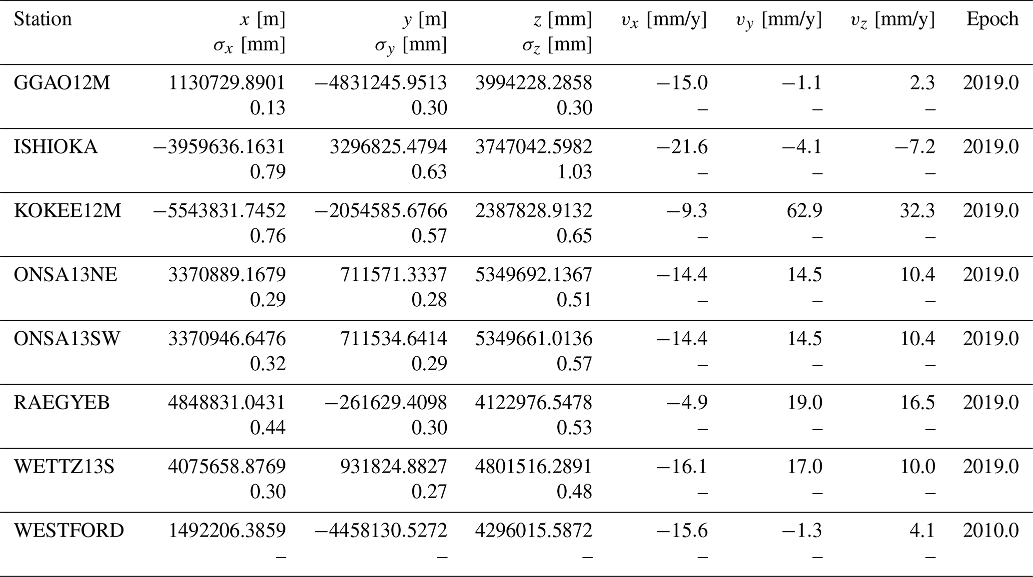
The VGOS station coordinates as determined with the best parametrization of the troposphere in a global solution are listed in Table 5 along with the formal errors σ. The velocities were not estimated but stem from co-located S/X stations as described in Sect. 3.1. In the case of ISHIOKA, the velocities were estimated from R1 and R4 S/X sessions in the time span 2017 to 2019.
The formal errors were obtained from the unconstrained least squares adjustment of the global solution. Therefore, they only capture the accuracy of the inner network geometry. In the chosen datum definition method, the EOP and WESTFORD coordinates are seen as true values and not as stochastic quantities during the adjustment. Inaccuracies in those values directly affect the estimated station coordinates but do not show up in the estimated formal errors. Additionally, errors in the a priori models pertaining to the station coordinates of WESTFORD also directly influence the estimation results. Therefore, the listed formal errors are too optimistic and not truly representative of the accuracies of the absolute positions of the estimated stations. More realistically, the absolute positional accuracy is at the few millimeter level.
This is confirmed by a comparison with ISHIOKA coordinates. While ISHIOKA is not listed in ITRF2014, the analysis of the S/X sessions also yielded coordinates that could be used for comparisons with VGOS data. The total length of the difference vector between the ISHIOKA positions from the two different solutions is close to 1 cm. However, ISHIOKA's accuracy might be comparatively worse, due to the limited number of sessions it participated in (see Fig. 1) and the fact that the long distance to WESTFORD accentuates the error caused by noise or possible biases in the EOP data.
Table 5The VGOS station coordinates resulting from the final global solution using the best parametrization for the tropospheric parameters and their formal uncertainties σ. The velocities v are taken from the ITRF2014 for co-located telescopes or were determined from X/S sessions in the case of ISHIOKA.
In this study we demonstrated how an unconstrained adjustment can be used for the definition of the geodetic datum of VLBI sessions to connect the VGOS network with the ITRF. Therefore, the station coordinates of WESTFORD and the five EOP were fixed to their a priori values. This approach was later used during a global solution of 30 VGOS sessions from 2017 and 2019 to estimate precise VGOS station coordinates.
In the future, it is assumed that the connection of the VGOS network to the ITRF will also be done based on local tie measurements and using local interferometer sessions. However, up to this point none of these results are publicly available. Additionally, within the IVS, three special sessions RD2005–RD2007 are planned where VGOS stations observe together with S/X stations in a mixed-mode. Results of these sessions will be most valuable to connect the VGOS network to the legacy S/X network. In 2021, several VGOS stations will be listed in ITRF2020, because the VGOS observations will be used for the generation of the next ITRF. After this point, the definition of the geodetic datum for VGOS sessions can be done using NNR and NNT conditions again.
In the course of this study, we also tested various parametrizations for the estimation of the tropospheric parameters in terms of baseline length repeatability values, because VGOS observations are expected to better resolve the troposphere at the stations. This investigation revealed that shorter estimation intervals for the gradients of 15 min and slightly longer estimation intervals of 45 min for the ZWD, compared to typical S/X analysis values, are beneficial. However, the ongoing maturing of VGOS, especially in terms of improvements in its scheduling (Schartner and Böhm, 2020), will likely continue to change the ideal parametrization of the tropospheric estimates.
The used VGOS data is publicly available from the Crustal Dynamics Data Information System (CDDIS DAAC; available at: https://cddis.nasa.gov/archive/vlbi/ivsdata/vgosdb/) (International VLBI Service for Geodesy and Astrometry, 2021).
MM analysed the VGOS sessions, implemented a unconstrained adjustment for global solutions in VieVS and tested different troposphere parametrizations. JB helped with the tropospheric parametrization while MS provided guidance for the unconstrained global solution. MM wrote the manuscript with input from JB and MS.
The authors declare that they have no conflict of interest.
This article is part of the special issue “European Geosciences Union General Assembly 2020, EGU Geodesy Division”. It is a result of the EGU General Assembly 2020, 4–8 May 2020.
The authors are grateful to the Austrian Science Fund (FWF) for supporting this work with project VGOS Squared (P 31625-N29).
We would like to thank all parties that contributed to the success of the CONT17 campaign, in particular to the IVS Coordinating Center at NASA Goddard Space Flight Center (GSFC) for taking the bulk of the organizational load, to the GSFC VLBI group for preparing the legacy S/X observing schedules and MIT Haystack Observatory for the VGOS observing schedules, to the IVS observing stations at Badary and Zelenchukskaya (both Institute for Applied Astronomy, IAA, St. Petersburg, Russia), Fortaleza (Rádio Observatório Espacial do Nordeste, ROEN; Center of Radio Astronomy and Astrophysics, Engineering School, Mackenzie Presbyterian University, Sao Paulo and Brazilian Instituto Nacional de Pesquisas Espaciais, INPE, Brazil), GGAO (MIT Haystack Observatory and NASA GSFC, USA), Hartebeesthoek (Hartebeesthoek Radio Astronomy Observatory, National Research Foundation, South Africa), the AuScope stations of Hobart, Katherine, and Yarragadee (Geoscience Australia, University of Tasmania), Ishioka (Geospatial Information Authority of Japan), Kashima (National Institute of Information and Communications Technology, Japan), Kokee Park (U.S. Naval Observatory and NASA GSFC, USA), Matera (Agencia Spatiale Italiana, Italy), Medicina (Istituto di Radioastronomia, Italy), Ny Ålesund (Kartverket, Norway), Onsala (Onsala Space Observatory, Chalmers University of Technology, Sweden), Seshan (Shanghai Astronomical Observatory, China), Warkworth (Auckland University of Technology, New Zealand), Westford (MIT Haystack Observatory), Wettzell (Bundesamt für Kartographie und Geodäsie and Technische Universität München, Germany), and Yebes (Instituto Geográfico Nacional, Spain) plus the Very Long Baseline Array (VLBA) stations of the Long Baseline Observatory (LBO) for carrying out the observations under the US Naval Observatory's time allocation, to the staff at the MPIfR/BKG correlator center, the VLBA correlator at Socorro, and the MIT Haystack Observatory correlator for performing the correlations and the fringe fitting of the data, and to the IVS Data Centers at BKG (Leipzig, Germany), Observatoire de Paris (France), and NASA CDDIS (Greenbelt, MD, USA) for the central data holds.
This research has been supported by the Austrian Science Fund (FWF) (grant no. P 31625-N29).
This paper was edited by Mathis Bloßfeld and reviewed by two anonymous referees.
Altamimi, Z., Rebischung, P., Métivier, L., and Collilieux, X.: ITRF2014: A new release of the International Terrestrial Reference Frame modeling nonlinear station motions, J. Geophys. Res.-Sol. Ea., 121, 6109–6131, https://doi.org/10.1002/2016JB013098, 2016. a
Bizouard, C., Lambert, S., Gattano, C., Becker, O., and Richard, J. Y.: The IERS EOP 14C04 solution for Earth orientation parameters consistent with ITRF 2014, J. Geodesy, 93, 621–633, https://doi.org/10.1007/s00190-018-1186-3, 2019. a
Böhm, J., Böhm, S., Boisits, J., Girdiuk, A., Gruber, J., Hellerschmied, A., Krásná, H., Landskron, D., Madzak, M., Mayer, D., McCallum, J., McCallum, L., Schartner, M., and Teke, K.: Vienna VLBI and Satellite Software (VieVS) for Geodesy and Astrometry, PASP, 130, 044503, https://doi.org/10.1088/1538-3873/aaa22b, 2018. a
Charlot, P., Jacobs, C. S., Gordon, D., Lambert, S., de Witt, A., Böhm, J., Fey, A. L., Heinkelmann, R., Skurikhina, E., Titov, O., Arias, E. F., Bolotin, S., Bourda, G., Ma, C., Malkin, Z., Nothnagel, A., Mayer, D., MacMillan, D. S., Nilsson, T., and Gaume, R.: The Third Realization of the International Celestial Reference Frame by Very Long Baseline Interferometry, Astron. Astrophys., submitted, 2020. a
Davis, J. L., Herring, T. A., Shapiro, I. I., Rogers, A. E. E., and Elgered, G.: Geodesy by radio interferometry: Effects of atmospheric modeling errors on estimates of baseline length, Radio Sci., 20, 1593–1607, https://doi.org/10.1029/RS020i006p01593, 1985. a
International VLBI Service for Geodesy and Astrometry: VGOSDB observation data, available at: https://cddis.nasa.gov/archive/vlbi/ivsdata/vgosdb/ (last access: 24 February 2021), NASA EOSDIS CDDIS DAAC, Greenbelt, MD, USA, 2021. a
Landskron, D. and Böhm, J.: VMF3/GPT3: refined discrete and empirical troposphere mapping functions, J. Geodesy, 92, 349–360, https://doi.org/10.1007/s00190-017-1066-2, 2018. a
Niell, A., Barrett, J., Burns, A., Cappallo, R., Corey, B., Derome, M., Eckert, C., Elosegui, P., McWhirter, R., Poirier, M., Rajagopalan, G., Rogers, A., Ruszczyk, C., SooHoo, J., Titus, M., Whitney, A., Behrend, D., Bolotin, S., Gipson, J., Gordon, D., Himwich, E., and Petrachenko, B.: Demonstration of a broadband very long baseline interferometer system: A new instrument for high‐precision space geodesy, Radio Sci., 53, 1269–1291, https://doi.org/10.1029/2018RS006617, 2018. a, b
Niemeier, W.: Ausgleichungsrechnung: Statistische Auswertemethoden, 2., De Gruyter, Berlin, Germany, 2008. a
Nilsson, T., Böhm, J., Wijaya, D. D., Tresch, A., Nafisi, V., and Schuh, H.: Path Delays in the Neutral Atmosphere, in: Atmospheric Effects in Space Geodesy, edited by: Böhm, J. and Schuh, H., Springer, Berlin, Heidelberg, 73–136, 2013. a
Nothnagel, A., Artz, T., Behrend, D., and Malkin, Z.: International VLBI Service for Geodesy and Astrometry, J. Geodesy, 91, 711–721, https://doi.org/10.1007/s00190-016-0950-5, 2017. a
Nothnagel A.: Very Long Baseline Interferometry, in: Handbuch der Geodäsie, edited by: Freeden W. and Rummel R., Springer Reference Naturwissenschaften, Springer Spektrum, Berlin, Heidelberg, https://doi.org/10.1007/978-3-662-46900-2_110-1, 2018. a
Petit, G. and Luzum, B.: IERS Conventions 2010, IERS Technical Note, 36, Verlag des Bundesamtes für Kartographie und Geodäsie, Frankfurt am Main, 2010. a
Petrachenko, B., Niell, A., Behrend, D., Corey, B., Böhm, J., Charlot, P., Collioud, A., Gipson, J., Haas, R., Hobiger, T., Koyama, Y., Macmillan, D., Malkin, Z., Nilsson, T., Pany, A., Tuccari, G., Whitney, A., and Wresnik, J.: Design Aspects of the VLBI2010 System, Progress Report of the IVS VLBI2010 Committee, Goddard Space Flight Center, Greenbelt, Maryland, available at: https://ivscc.gsfc.nasa.gov/publications/misc/TM-2009-214180.pdf (last access: 24 February 2021), 2009. a, b
Plank, L., Lovell, J. E. J., Shabala, S. S., Böhm, J., and Titov, O.: Challenges for geodetic VLBI in the southern hemisphere, Adv. Space Res., 56, 304–313, https://doi.org/10.1016/j.asr.2015.04.022, 2015. a
Saastamoinen, J.: Atmospheric Correction for the Troposphere and Stratosphere in Radio Ranging Satellites, in: The Use of Artificial Satellites for Geodesy, edited by Henriksen, S. W., Mancini, A., and Chovitz, B. H., 15, 247–251, AGU, Washington, D.C., 1972. a
Schartner, M. and Böhm, J.: Optimizing schedules for the VLBI global observing system, J. Geodesy, 94, 12, https://doi.org/10.1007/s00190-019-01340-z, 2020. a, b
Schuh, H. and Böhm, J.: VLBI for Geodesy and Astrometry, in: Sciences of Geodesy II, Innovations and Future Developments, edited by: Xu, G., Springer, Berlin, 2013. a, b, c