 | 19 Oct 2020
Modelling ground displacement and gravity changes with the MUFITS simulator
Ivan Utkin
We present an extension of the MUFITS reservoir simulator for modelling the ground displacement and gravity changes associated with subsurface flows in geologic porous media. Two different methods are implemented for modelling the ground displacement. The first approach is simple and fast and is based on an analytical solution for the extension source in a semi-infinite elastic medium. Its application is limited to homogeneous reservoirs with a flat Earth surface. The second, more comprehensive method involves a one-way coupling of MUFITS with geomechanical code presented for the first time in this paper. We validate the accuracy of the development by considering a benchmark study of hydrothermal activity at Campi Flegrei (Italy). We investigate the limitations of the first approach by considering domains for the geomechanical problem that are larger than those for the fluid flow. Furthermore, we present the results of more complicated simulations in a heterogeneous subsurface when the assumptions of the first approach are violated. We supplement the study with the executable of the simulator for further use by the scientific community.
- Article
(5163 KB) - Full-text XML
- BibTeX
- EndNote


Reservoir simulation remains an essential area for forecasting various parameters of subsurface exploration and natural flows. The capabilities of the reservoir simulators, i.e., the computer programs for modelling the flows in geologic porous media, are constantly improving. The modern simulators can account for additional physical phenomena and technological processes. For example, the modelling of Darcy flows is often coupled with rather sophisticated approaches for geomechanics, multiphase transport in wellbores, and other processes (Fig. 1). More common in petroleum reservoir simulation is the development and utilisation of universal software packages allowing for conveniently integrated workflows for coupled thermo-hydro-mechanical modelling and history matching of the models (Fanchi, 2006).
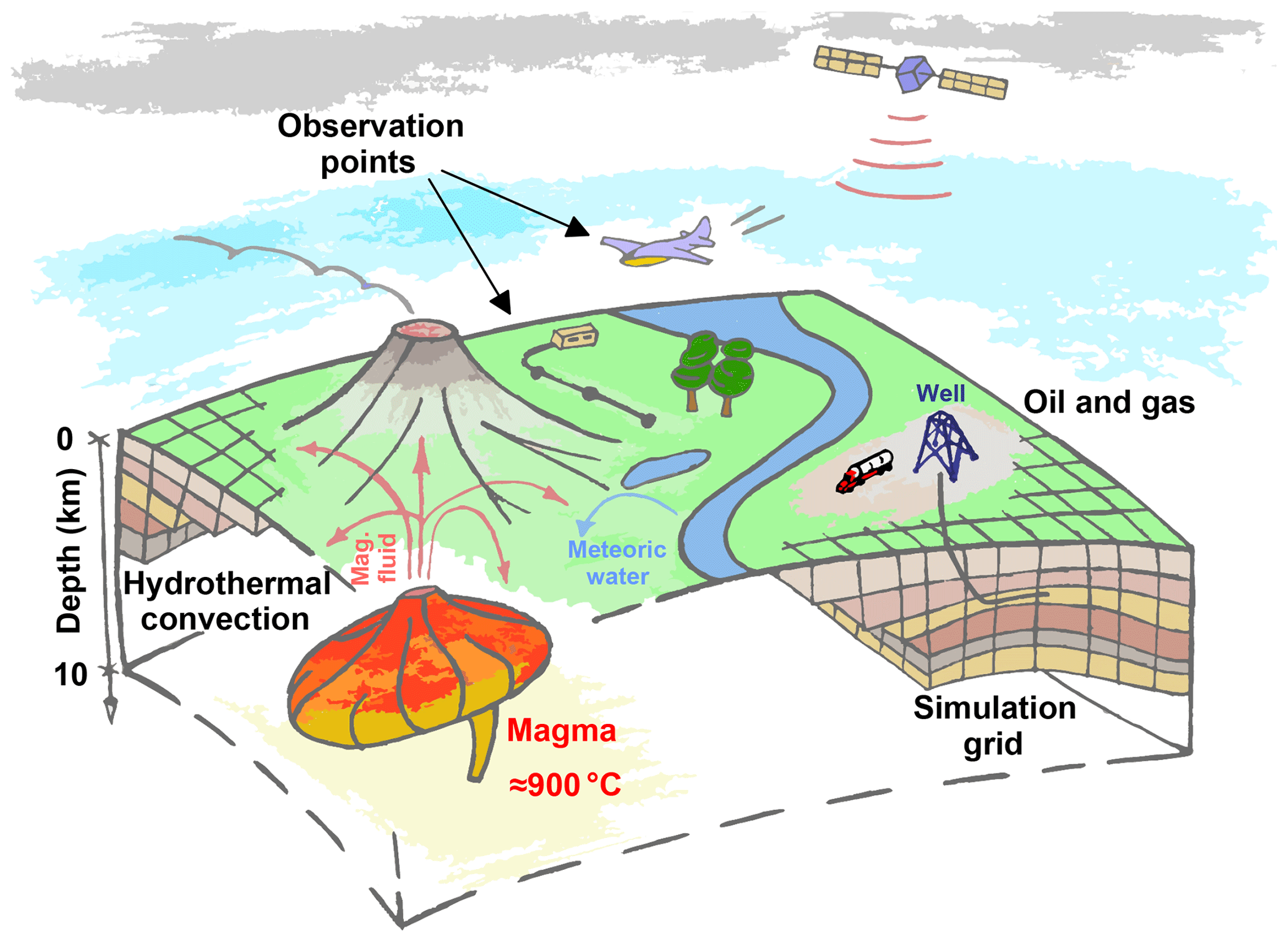
Figure 1Sketch of typical processes in hydrothermal systems (left) and petroleum reservoirs (right). Magma degassing results in a plume of hot magmatic fluid. Near the surface, the fluid can mix with colder meteoric water. The observation points, where the ground displacement and gravity changes can be measured, are shown.
The numerical modelling of hydrothermal systems differs in several respects from that of petroleum reservoirs (Fig. 1). First, the flows occur under a much wider range of temperatures. This necessitates the application of sophisticated models accounting for phase transitions and reactive transport under both low and high temperatures. Also, the plastic deformations of rocks in the brittle-ductile transition zone of hydrothermal systems should be considered. Secondly, the transport in hydrothermal systems, especially the natural one, can be observed through a very limited number of parameters. Usually, only observations at the surface are available. This is incomparable with petroleum reservoirs, where many more observable parameters are available through extensive drilling and seismic studies. The parameters of heat and mass transfer in hydrothermal systems can be estimated by measuring the surface fluxes of magmatic gas and heat. Also, the parameters of the flows can be estimated by measuring the gravity changes and ground displacement. The periods of unrest of more intense magma degassing into overlying rocks can result in the fluid density increasing in extended regions leading to significant gravity changes at the surface, which can be observed by gravimeters mounted on the surface or aircraft (Fig. 1). Similarly, the redistribution of strains and stresses causes significant ground displacement that can reach tens of centimeters in particular cases (Chiodini et al., 2003; Hurwitz et al., 2007; Hutnak et al., 2009; Rinaldi et al., 2010). Such values of the ground uplift (or subsidence) can be observed by either surface measurements or satellite radar interferometry.
In the numerical modelling of hydrothermal systems, a common approach for estimating gravity changes and ground displacement assumes the application of different computer programs that are not directly compatible with each other. The fluid flow is simulated by using hydrodynamic code. Then, the gravity changes are calculated by post-processing the simulation results in separate code, i.e., by summing the contributions of every grid block to the strength of the gravitational field (Todesco, 2009). Such calculations, although very straightforward, can require a significant effort to develop the interface between the computer programs. A similar approach based on summing the contributions of the grid blocks to the magnitude of ground displacement exists for predicting the subsidence or uplift of Earth's surface (Rinaldi et al., 2011). It also requires considerable efforts to post-process the simulation results. For ground displacement, a more comprehensive approach assumes the coupling of hydrodynamic and geomechanical simulators, which again requires time-consuming efforts to program the interface between the simulators (Todesco et al., 2004; Rutqvist, 2011). Therefore, simulation software allowing for all the calculations described above in an integrated framework is in demand. The goal of this work is the development of such software by extending MUFITS. We supplement the simulator with built-in capabilities for calculating gravity changes and ground displacement and verify the development against a benchmark study.
2.1 Review of the simulator and new developments
MUFITS has been developed over the past decade. Initially, it was designed for modelling the subsurface storage of CO2 in saline aquifers and petroleum reservoirs at relatively low temperatures (Afanasyev, 2013, 2015). Then, it was extended for the modelling at much higher reservoir temperatures including supercritical parameters. The simulator was applied for modelling the natural convection at Campi Flegrei caldera down to a depth of 5 km (Afanasyev et al., 2015). A 3-D model of the subsurface near the Solfatara crater was created and calibrated against the measurements of the surface fluxes of magmatic gas and heat as well as the temperature profiles in a few boreholes. Also, MUFITS was applied to the investigation of the high-temperature flows in the kimberlite pipes during their cooling (Afanasyev et al., 2014) and the formation of lenses of hypersaline fluid above degassing magma bodies (Afanasyev et al., 2018). Until now, the functionality of the simulator did not allow for easy computations of gravity changes and ground displacement, which could help in a better understanding of the flows in the described applications and more reliable history matching of the corresponding reservoir models. The development of such a functionality would be a good step towards transforming MUFITS into a universal software package for modelling hydrothermal systems.
As presented in Sect. 2.3, MUFITS now allows for the built-in calculation of gravity changes. The developed extension of the software includes two methods, A and B, for calculating ground displacement (Fig. 2). Option A is built into the hydrodynamic simulator. It employs an analytical solution for the extension source in a semi-infinite elastic medium corresponding to Earth's subsurface. Every grid block is considered such a point source, and the ground displacement is calculated by summing the contributions of all grid blocks, as described in Sect. 2.4. Thus, method A does not require any interface between hydrodynamics and geomechanics, because it is built into the hydrodynamic code. Option B assumes that MUFITS is coupled with geomechanical code through external files. Now, MUFITS is supplemented with Matlab code for axisymmetric modelling the distributions of strains and stresses and a command-line tool (an external script) that converts MUFITS output files into a simpler binary format readable by Matlab. This tool allows Matlab code to read the external files produced by MUFITS; thus, additional efforts for programming the interface are not needed. Furthermore, this open-source tool can be useful for a quick MUFITS coupling with other software. The equations implemented in the geomechanical code are discussed in Sect. 3.

Figure 2Diagram showing the software options for modelling gravity changes and ground displacement. The interface between the simulators is organised through external files.
2.2 Observation points
To extend MUFITS for the modelling of gravity changes and ground displacement, a new primitive (element) of the reservoir model, namely the “observation point” (OP), is introduced. Every OP is assigned a character name and is characterised by 3 coordinates in space. For example, an OP can correspond to surface or airborne measurements (Fig. 1). The simulator can be set up for automated calculation of the gravity changes and ground displacement in every OP at every moment of time. To ease the reporting of space distributions, OPs can be grouped into networks of equally spaced points along the x, y, and z axes.
The developed options for simulating gravity changes and ground displacement (by method A) are generally designed for 3-D simulations with domains of arbitrary complexity (Fig. 3a). However, a domain symmetry can often be implied in 2-D simulations to speed them up. The influence of the symmetries on parameters in an OP can automatically be accounted for in the following cases. First, axisymmetric simulations are allowed when the flow is calculated only in a fraction of the full circle (corresponding to the opening angle φ). In this case, the x and y coordinates of a point E belonging to the vertical axis of rotation must be specified (Fig. 3b). Secondly, translational symmetry of the domain is allowed when the 2-D flow is calculated only in a plane fraction (of thickness h) of the 3-D space (Fig. 3c). In this case, the x and y coordinates of the horizontal translational vector nt must be specified. Thirdly, in addition to the previous option, reflection symmetry is allowed by specifying a point B belonging to the reflection plane and the normal to the plane nb (Fig. 3d). For these symmetries, the simulator can automatically account for other parts of 3-D space that do not belong to the domain.
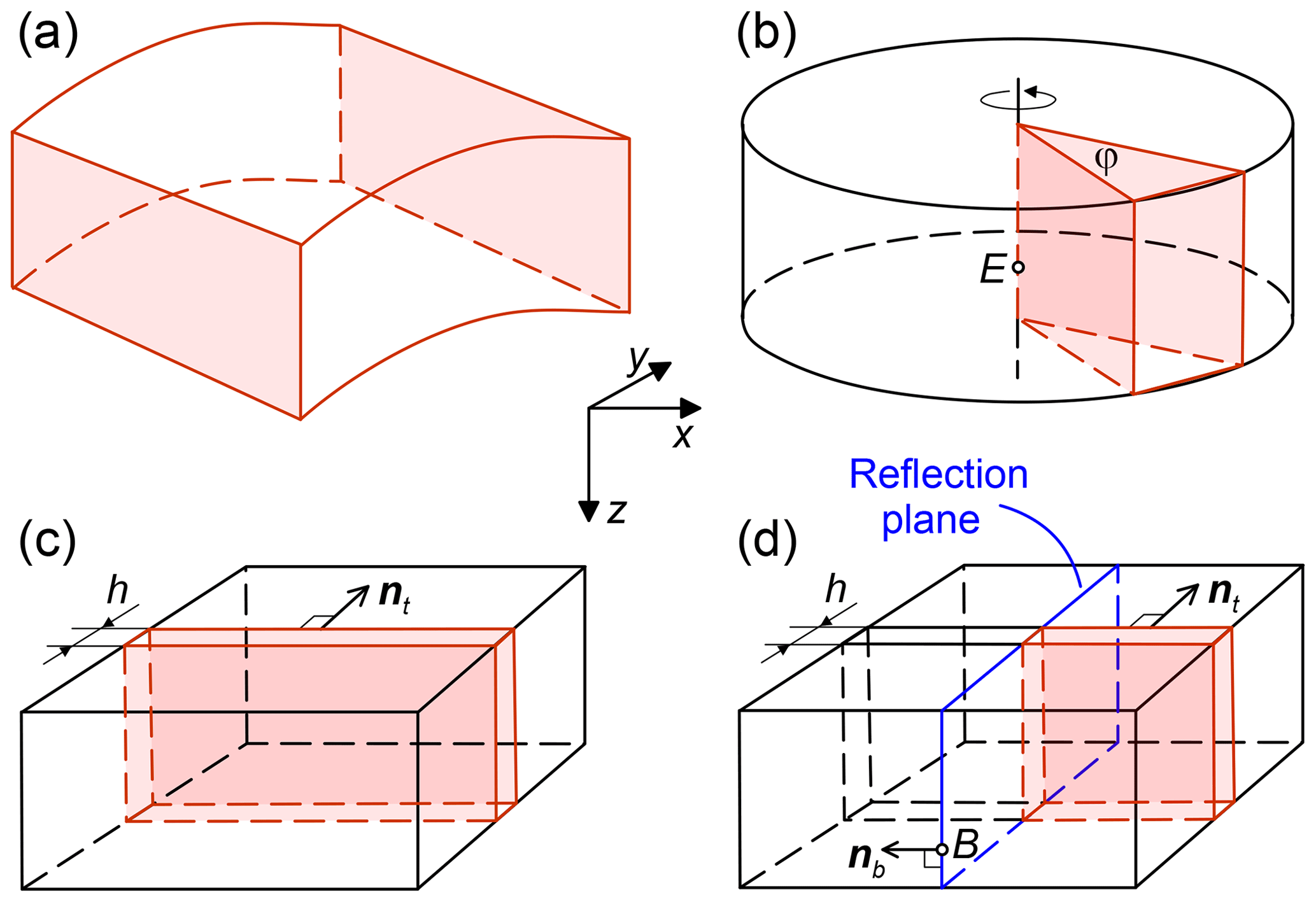
Figure 3Possible symmetries that can be accounted for in the calculation of gravity changes and ground displacement by method A. The simulation domain (red) occupies a region of the subsurface reservoir (black).
We denote by and the position vectors of an OP and a grid block centre, respectively. In accordance with the finite volume method implemented in MUFITS, the gravity changes and ground displacement in an OP are calculated by summing the contributions of every grid block to the magnitudes of these fields. Herewith, the finite size of the blocks is neglected by considering them as point sources placed at ri. The corresponding equations are discussed below.
2.3 Modelling gravity changes
According to Newton's law of universal gravitation, the gravity change in every OP is calculated using the following equation:
where Δg is the gravity change, N is the number of grid blocks in the simulation, γ is the gravity constant, ρ is the bulk density of the saturated porous medium, ρ0 is the reference bulk density, V is the volume of a grid block, and the subscript i denotes the parameters of the ith block. The change Δg is calculated against the reference state with distribution of density ρ0. By default, the distribution of ρ at the initial moment of time is set as the reference distribution ρ0. However, the user can override this setting by specifying moments of time at which the distribution of ρ is copied to ρ0. Thus, one can choose (or redefine) the moment of time of the reference state.
2.4 Modelling ground displacement (method A)
Method A is restricted by the following assumptions:
-
The mechanical properties of the saturated porous medium are homogeneous.
-
The top boundary of the domain, z=ztop, corresponding to Earth's surface, is flat, horizontal, and free of stresses.
-
The domain for modelling the displacement is a semi-infinite region z≥ztop filled with an elastic medium.
Given that these assumptions are satisfied, the displacements are calculated by employing an analytical solution for the centre of compression (or dilatation) placed in the interior of the semi-infinite solid (Mindlin, 1936; Mindlin and Cheng, 1950). Every grid block is considered such a centre of compression, and the relative change in the grid block volume is calculated as (Rinaldi et al., 2010)
where P and T are the pressure and temperature, P0 and T0 are their values in the reference state, is the change in grid block volume against the reference state, 1∕H is Biot's constant, K is the isothermal drained bulk modulus, Ks is the bulk modulus of the solid phase, and αs is the volumetric thermal expansion coefficient.
Using the analytical solution of Mindlin and Cheng (1950), the displacement in every OP is calculated as:
where is the displacement and the following notations are introduced:
Here, ν and μ are Poisson's ratio and the shear modulus, respectively. Equations (3) and (4) are those presented by Rinaldi et al. (2010) with the exception of the sign of the second term within the brackets in Eq. (3).
The displacement u is calculated against the reference state characterised by the distributions of pressure P=P0 and temperature T=T0. By default, the distributions of P and T at the initial moment of time are set as the reference. This setting can be overridden by specifying the moments of time at which MUFITS copies the distributions of P and T to P0 and T0, respectively. Thus, one can choose (or redefine) the moment of time of the reference state.
Method A provides a fast option for calculating ground displacement. However, this mathematical model is restricted to the case of a homogeneous distribution of thermoporoelastic moduli and is subject to other assumptions described in Sect. 2.4. This limits the range of potential applications of the built-in ground deformation model. Several studies (Trasatti et al., 2005; Chiarabba and Moretti, 2006; Manconi et al., 2010) show that the mechanical properties of rocks within hydrothermal systems can exhibit significant heterogeneity, which method A cannot deal with.
To allow for the modelling of hydrothermal systems with heterogeneous mechanical properties, we have developed numerical code for calculating stresses and displacements by the finite volume method in axisymmetric domains. The solution of the elastic problem is uncoupled from the equations governing the fluid flow, i.e., deformations of the solid phase do not influence the fluid pressure or the porosity and permeability of the rock matrix. This is justified by the assumption of small deformations. In addition, uncoupling the ground displacement from the fluid flow makes it possible to implement method B in a post-processing module of the simulator, removing the necessity to re-run MUFITS simulations in order to change the mechanical properties of the rocks.
The constitutive equations for linear isotropic thermoporoelastic medium are expressed as (Coussy, 2004)
Here, Ptot and τij are the hydrostatic and deviatoric components of the total stress tensor , εij is the infinitesimal strain tensor, b is the Biot–Willis coefficient, and the subscript 0 denotes the quantities in the reference state.
We seek a numerical solution of the equations of static equilibrium:
There is no gravity contribution in Eq. (6) because we consider the deviations of stresses and displacements from the reference state. For axisymmetric problems, system (6) is solved in a cylindrical coordinate system , and the displacements in the direction of the angular coordinate, uφ, are assumed to be zero. For 2-D problems formulated in Cartesian coordinates, system (6) is solved under conditions of plane strain.
The equations of elastic equilibrium (6) are integrated using the pseudo-transient (PT) method (Duretz et al., 2018). In accordance with this method, instead of solving the elliptic problem directly, which usually requires assembling matrices for a discretised system, the pseudo-time derivative is added to the right-hand side of Eq. (6). Then, the system is advanced in pseudo-time from some initial distribution of the parameters until it reaches a steady state.
The advantages of the PT method in comparison to other numerical techniques that require assembling matrices are the brevity of the corresponding code and the simplicity of its development and modification. However, since the PT method involves only explicit time integration, the number of iterations required for convergence scales quadratically with the number of grid blocks due to stability conditions. This is acceptable only for 1-D problems and can be too restrictive for 2-D and 3-D problems. To overcome this limitation and accelerate convergence, we use the second-order pseudo-transient method (Räss et al., 2019), which implies adding both first and second time derivatives to the right-hand side of Eq. (6). The second-order PT method is mathematically equivalent to the method of successive over-relaxation (Frankel, 1950).
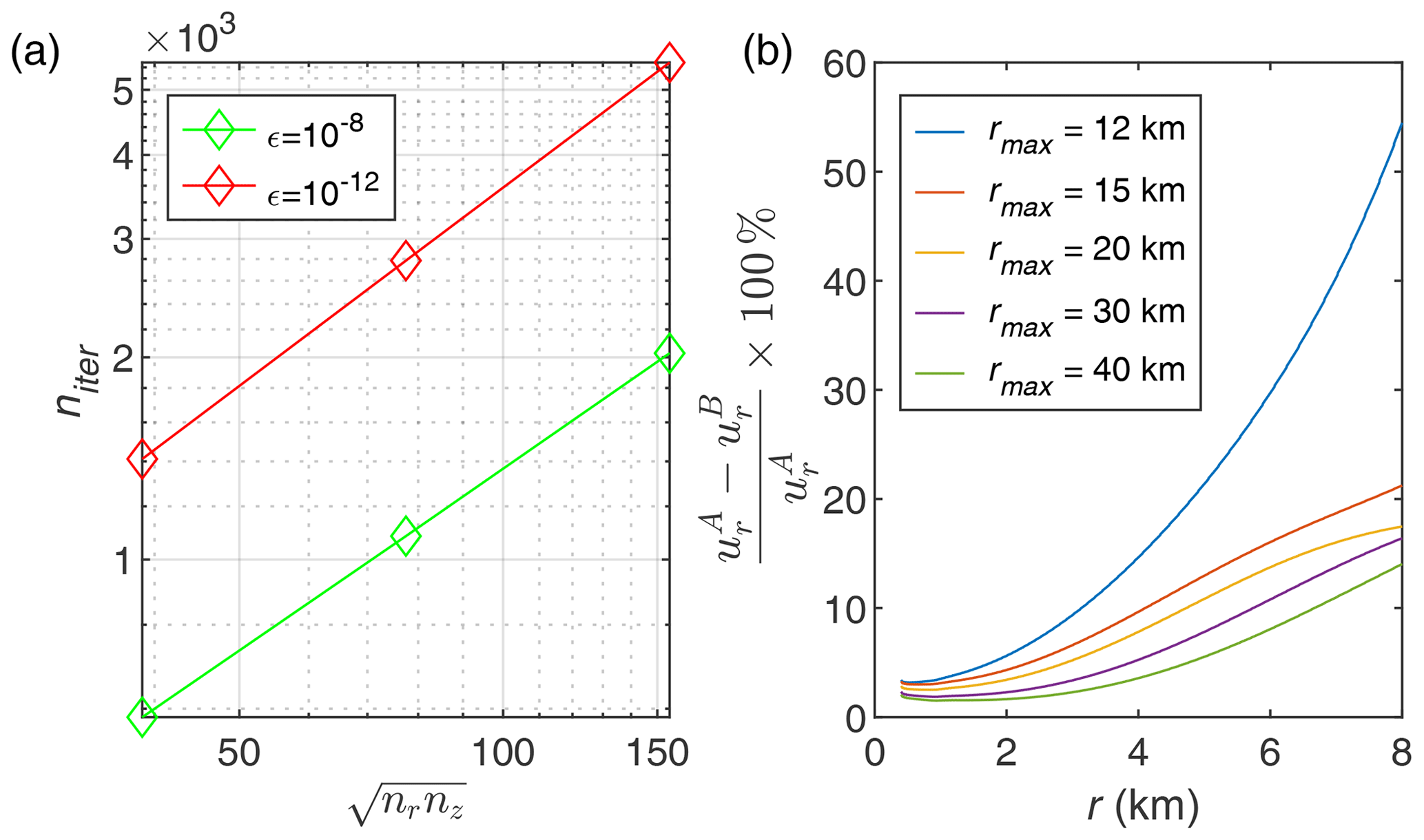
Figure 4Average number of pseudo-transient iterations niter required to satisfy different convergence criteria ϵ (a) and relative deviation of the radial component of displacements calculated with method B () from those calculated using method A () for various grid extension factors (b).
As shown in Fig. 4a, the second-order PT method scales linearly with problem size which is sufficient for the present study. In all benchmarks considered in the subsequent sections, the total computation time of geomechanical code doesn't exceed 10 % of the running time of the hydrodynamic code, if the same hardware is used both for MUFITS and the code implementing method B.
4.1 Problem statement for the hydrodynamic modelling
To validate the developed modelling options, we consider an axisymmetric study of hydrothermal activity at Campi Flegrei, a caldera located in southern Italy. An accelerated ground deformation and heating is observed in this densely populated area of Naples causing interest to understanding and predicting the hydrothermal activity. The corresponding flows in the hydrothermal system and associated observable parameters at the surface were broadly investigated by Chiodini et al. (2003, 2016), Todesco et al. (2003, 2004), Todesco (2009), Rinaldi et al. (2010, 2011), Troiano et al. (2011), and Coco et al. (2016) among others. Thus, the parameters of the hydrothermal activity are well constrained, and they can be used for benchmarking. In this paper, we consider the problem statement that is most consistent with that described by Rinaldi et al. (2011).
We simulate the non-isothermal flow of a CO2–H2O binary mixture in the axisymmetric domain km, km, where r is the distance to the axis of rotation and z is the depth (Fig. 5). The domain near r=0 corresponds to the region below the Solfatara crater. At the initial moment of time, years, the homogeneous porous medium is saturated with pure water under a hydrostatic distribution of P and a linear distribution of T corresponding to a geothermic gradient of 50 ∘C km−1. A fixed atmospheric pressure and temperature, Patm=1 bar and Tatm=20 ∘C, are imposed at the opened upper boundary corresponding to Earth's surface. The system can be recharged with pure H2O through z=0. The constant T of 95 ∘C, which is consistent with the geothermic gradient and Tatm, is maintained at the impermeable lower boundary z=1.5 km. The side boundary r=10 km is impermeable and adiabatic. The simulation results indicate that the conditions at r=10 km do not influence the flow near r=0.
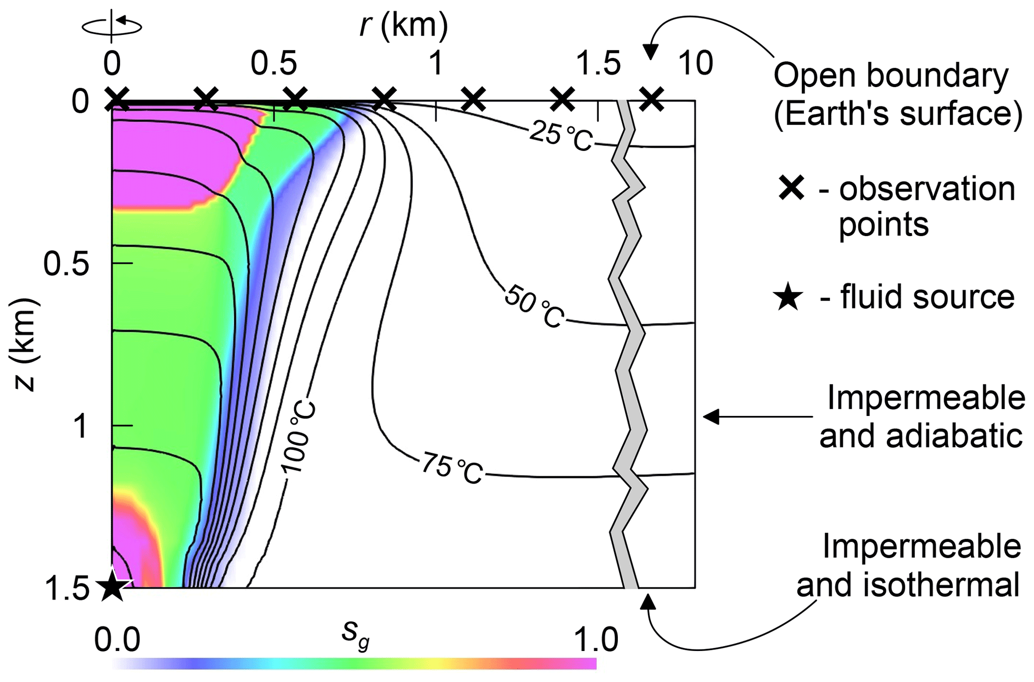
Figure 5The simulation domain and the boundary conditions for the hydrodynamic simulation. The distribution of the gas saturation (sg) and the isotherms are shown at t=120 months.
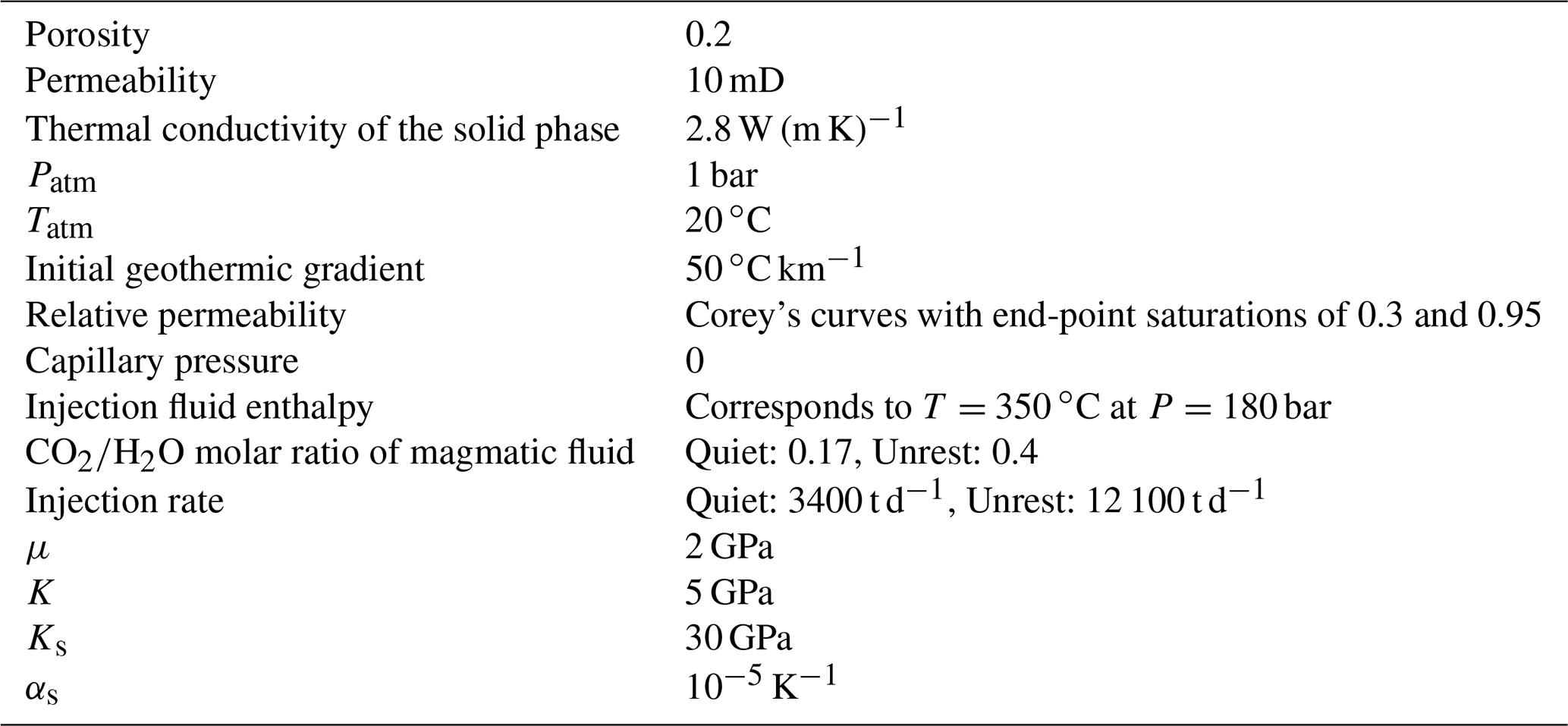
The influx of fluid from a deep magmatic source is simulated with a point source placed at r=0 km and z=1.5 km (Fig. 5). A hot mixture of CO2 and H2O, which should be regarded as a proxy for magmatic fluid, is injected into the domain through this source. The mixture enthalpy corresponds to T=350 ∘C at P=180 bar. The pressure near the fluid source increases up to ≈180 bar; thus, the temperature near the source is close to 350 ∘C. Consequently, it is assumed that the domain includes only a region above the brittle-ductile transition, where T does not exceed 350 ∘C (Hayba and Ingebritsen, 1997). Therefore, we consider only elastic deformations of the saturated rocks. First, we simulate 4000 years of degassing with a constant injection rate of 3400 t d−1 and a CO2∕H2O molar ratio of 0.17 (i.e., the molar concentration of CO2 is 0.1453). This interval is considered to be a period of dormancy over which a quasi-steady state is reached. After 4000 years, the plume of hot fluid forms near the axis of rotation r=0. It contains two distinct gas zones: one near the injection point and the other at shallow depths. Then, we simulate an event of unrest by temporally increasing the injection rate to 12 100 t d−1 and the CO2∕H2O molar ratio to 0.4. The unrest begins at t=0 and lasts over 20 months. After the unrest, at t=20 months, the point source is returned to the quiet state by reducing the injection rate and the molar ratio to their initial values. Other parameters of the study are summarised in Table 1.
For modelling the non-isothermal flow associated with the formation of the plume of hot magmatic fluid, we use a standard system of governing equations. It includes the continuity equations for CO2 and H2O, the heat equation, and Darcy's law. The governing equations are described in Afanasyev et al. (2015). They are identical to those used by Chiodini et al. (2003), Todesco (2009), Rinaldi et al. (2011), and others. The only difference is the approach for predicting the vapor-liquid equilibria and the parameters of the fluid phases for the CO2–H2O mixture. Chiodini et al. (2003), Todesco (2009), and Rinaldi et al. (2011) applied the TOUGH2/EOS2 simulator (Pruess et al., 1999), which up to the critical point of H2O employs Henry's law for the solubility of CO2 in liquid and other empirical correlations. Unlike them, we apply a fully consistent thermodynamic model of the mixture based on a cubic equation of state (EoS). The EoS is used for predicting both the mutual solubilities of CO2 and H2O and the phase densities and enthalpies in the whole range of P and T occurring in the study. The details of the EoS and the discussion of its accuracy can be found in Afanasyev et al. (2015).
We use radial non-uniform grids with the r and z factors equal to 1.025 and 1.05, respectively. Thus, the grids become denser near the axis of rotation (r=0) and the surface (z=0) to better resolve the plume. We consider grids 1X (45×8), 2X (60×15), 4X (90×30), etc., where the number of grid blocks along the r and z axes, nr×nz, are given in the brackets, respectively. The thickness of the grid blocks is less than 5 m in the case of the most refined grid, 12X (160×90).
For modelling the gravity changes and ground displacement by method A, we specify a network of equally spaced OPs along the straight line z=0 (Fig. 5). The simulator automatically calculates Δg and u for every OP in the network at every moment of time in accordance with the problem symmetry shown in Fig. 2b. Only one OP placed at r=0 and z=0 is needed for reporting the temporal evolution of Δg and u at the axis of rotation (i.e., at Solfatara). All OPs are used for reporting the space distributions of Δg and u at a fixed moment of time. The distributions of P, T, and the bulk density ρ at the beginning of the unrest (at t=0) are chosen as the reference values P0, T0, and ρ0 in Eqs. (1)–(3), (5), and (6).
4.2 Problem statement for the geomechanical modelling (method B)
We apply an extended grid to reduce the influence of the boundary conditions on the elastic equilibrium (Fig. 6). This makes possible the comparison and additional validation of methods A and B. For Eq. (6), we consider the domain , , where km and km. The traction-free condition, , is imposed at the upper boundary z=0, where n is the normal to the boundary. The “roller” boundary condition, , is imposed at the lower and side boundaries, and . When modelling the ground displacement, we account for the fluid pressure and temperature changes only in the region km, km, where the fluid flow is simulated. The changes in P and T are assumed to be zero outside this region.

Figure 6The domain and the boundary conditions for the geomechanical simulation by method B. The mesh used for the fluid flow modelling is shown in black. The distribution of total displacement is shown at t=20 months.
If the domains for the hydrodynamic and geomechanical modelling coincide, i.e., km and km, then the displacements u calculated by methods A and B differ significantly. This is explained by the influence of the boundary conditions at and on u near r=0 because they are not consistent with the assumption of the semi-infinite domain z≥0. If the boundaries are set progressively farther away from the centre region, i.e., km and km, then their influence on u decreases. We investigated optimal values of rmax and zmax that allow for the simulations to be consistent with the assumptions in Sect. 2.4 without excess computational cost. The investigation shows that a three times larger domain along both the r and z axes produces a satisfactory agreement between methods A and B (Fig. 4b). Thus, km and km are used in the following presentation. Herewith, the mesh outside the domain for hydrodynamic modelling should not be very dense. A coarse grid such as that shown in Fig. 6 is sufficient, and further grid refinement doesn't change the displacements in the region of interest.
4.3 Simulation results
The vertical components of the gravity change and ground displacement, Δgz and uz, at r=0, z=0 against t are shown in Fig. 7. The positive (or negative) values of uz correspond to the surface uplift (or subsidence). The positive Δgz corresponds to the elevated gravity field as compared to the reference state. Over the unrest, the average pressure and temperature as well as the bulk density increase because the hydrothermal system is inflated at the higher injection rate. As a consequence, the surface rises by about uz=10 cm and the gravity increases by Δgz=20 µGal. Then, as the fluid source reverts to the quiet state, uz and Δgz decrease because the fluid evaporates and is released through the upper boundary z=0, leading to a reduction in pressure and bulk density. The quantity Δgz reaches a minimum of −120 µGal at t=75 months and then increases back to 0 as the system returns to the quasi-steady state.
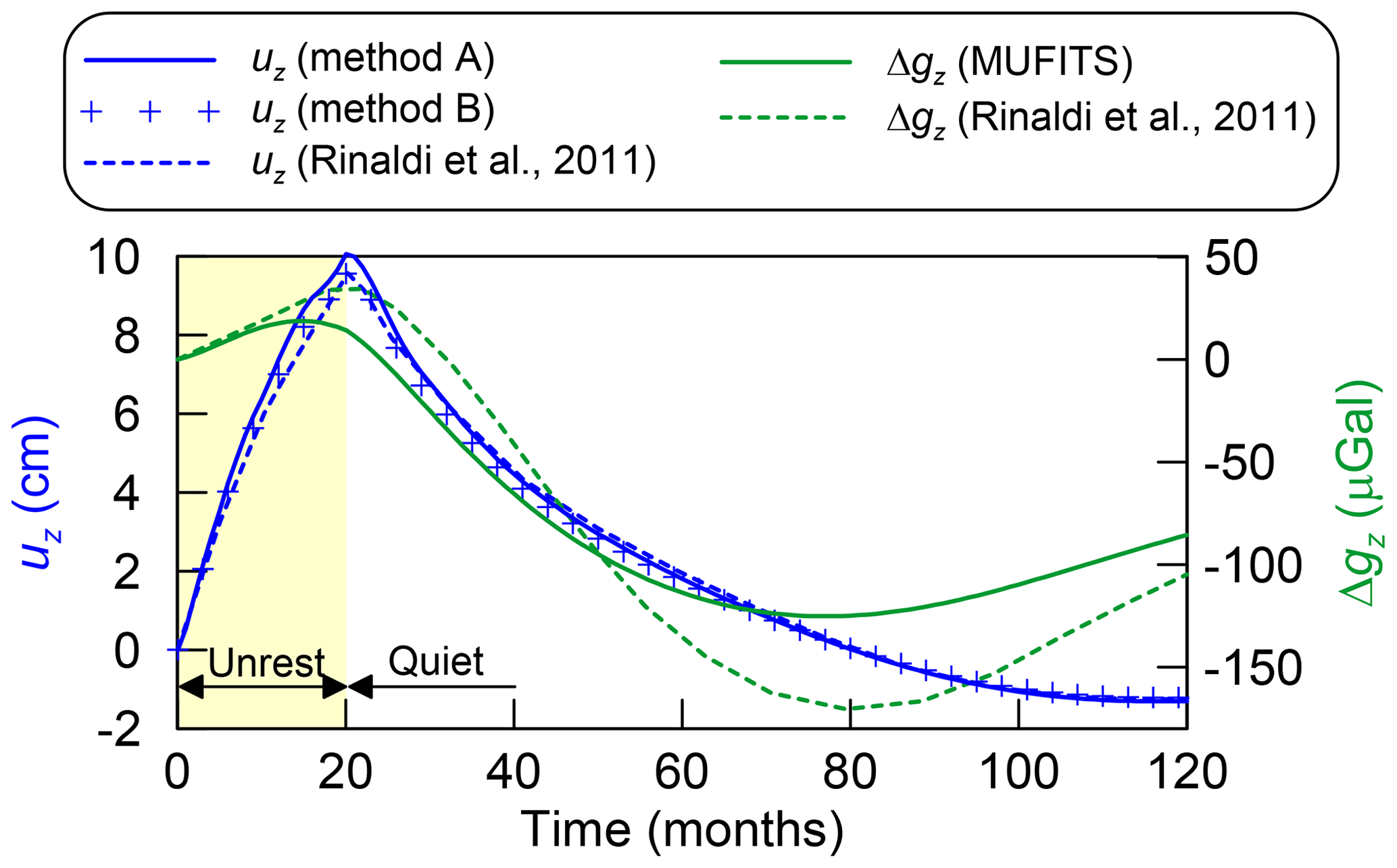
Figure 7Vertical components of the ground displacement (uz) and gravity change (Δgz) at the centre OP (r=0, z=0) against time.
An agreement between the u values predicted by methods A and B and those reported by Rinaldi et al. (2011) validates the correctness of the numerical algorithms implemented for modelling the ground displacement (Figs. 7 and 8). In general, Δgz changes with time similarly to that in Rinaldi et al. (2011). The intervals of Δgz increase and decrease are identical. However, the absolute values of Δgz are almost 1.5 times smaller than those reported by Rinaldi et al. (2011). This discrepancy can be caused by different EoS for the CO2–H2O mixture implemented in MUFITS and TOUGH2/EOS2. The different approaches for predicting the fluid properties can result in slightly different distributions of the bulk density (ρ) and, thus, the gravity change (Δg).
The results shown in Figs. 7 and 8 are simulated using the 4X grid (see Sect. 4.1). This choice is based on the mesh dependency study, the results of which are presented in Fig. 9. The utilisation of coarse grids, such as 1X and 2X, results in a slight underestimation of both ur and uz. The values of ur and uz become higher with increasing grid resolution. The convergence is achieved for the 8X grid, and further refinement is not needed. However, u for the 4X grid is satisfactorily close to that for 8X (and 12X) and can be used to reduce the computational cost. Thus, the simulations using method B were performed only for the grid resolutions up to 4X, as shown in Fig. 9c, d.
The results of Rinaldi et al. (2011) are in between our simulation results with the 2X and 4X grids (Fig. 9a, b). Presumably, this is caused by different methods for predicting the fluid properties employed in TOUGH2/EOS2 simulator, which up to the critical point of H2O employs Henry's law for the solubility of CO2 in liquid, and MUFITS, which employs a fully consistent thermodynamic model based on a cubic equation of state (EoS). Consequently, the distributions of P, T, and u obtained in this study can be slightly different from those in Rinaldi et al. (2011). However, the distributions are identical in qualitative sense confirming the correctness of the algorithms implemented in MUFITS.
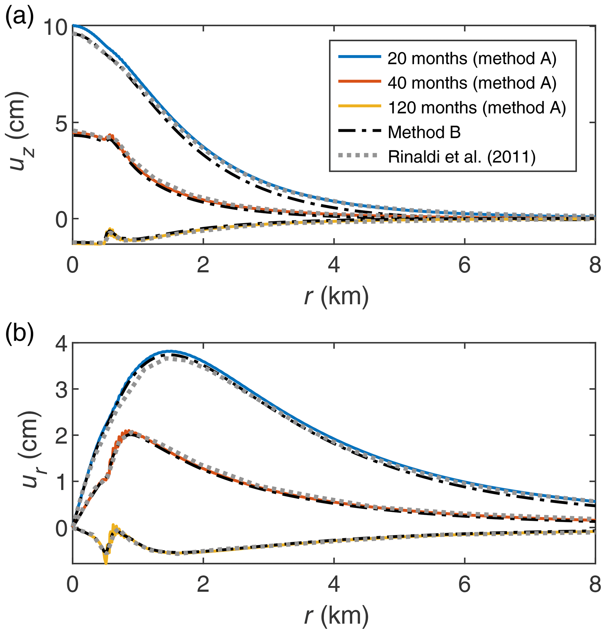
Figure 8Radial distribution of the vertical (a) and horizontal (b) ground displacement at sequential times. The coloured and dash-dotted lines correspond to methods A and B, respectively.
The distribution of u calculated by method A exhibits an oscillatory behaviour near the maximum of ur (Fig. 9b). Such an artificial oscillation is caused by the space discretisation of the domain and the finite volume method. When Eqs. (2)–(4) are applied, the changes in Pi and Ti in a grid block, which are distributed continuously over the entire grid block, are pulled to its centre to produce the point source of extension. Therefore, if the OP is closer to such a nearby centre in the uppermost row of grid blocks (i.e. if R1 and R2 are smaller), then u is higher than if the OP is between such centres (i.e. if R1 and R2 are larger). This results in the oscillatory behaviour because, according to Eqs. (2)–(4), there is inverse relationship between u and R1 (and R2). The quantity Δg can exhibit similar behaviour.
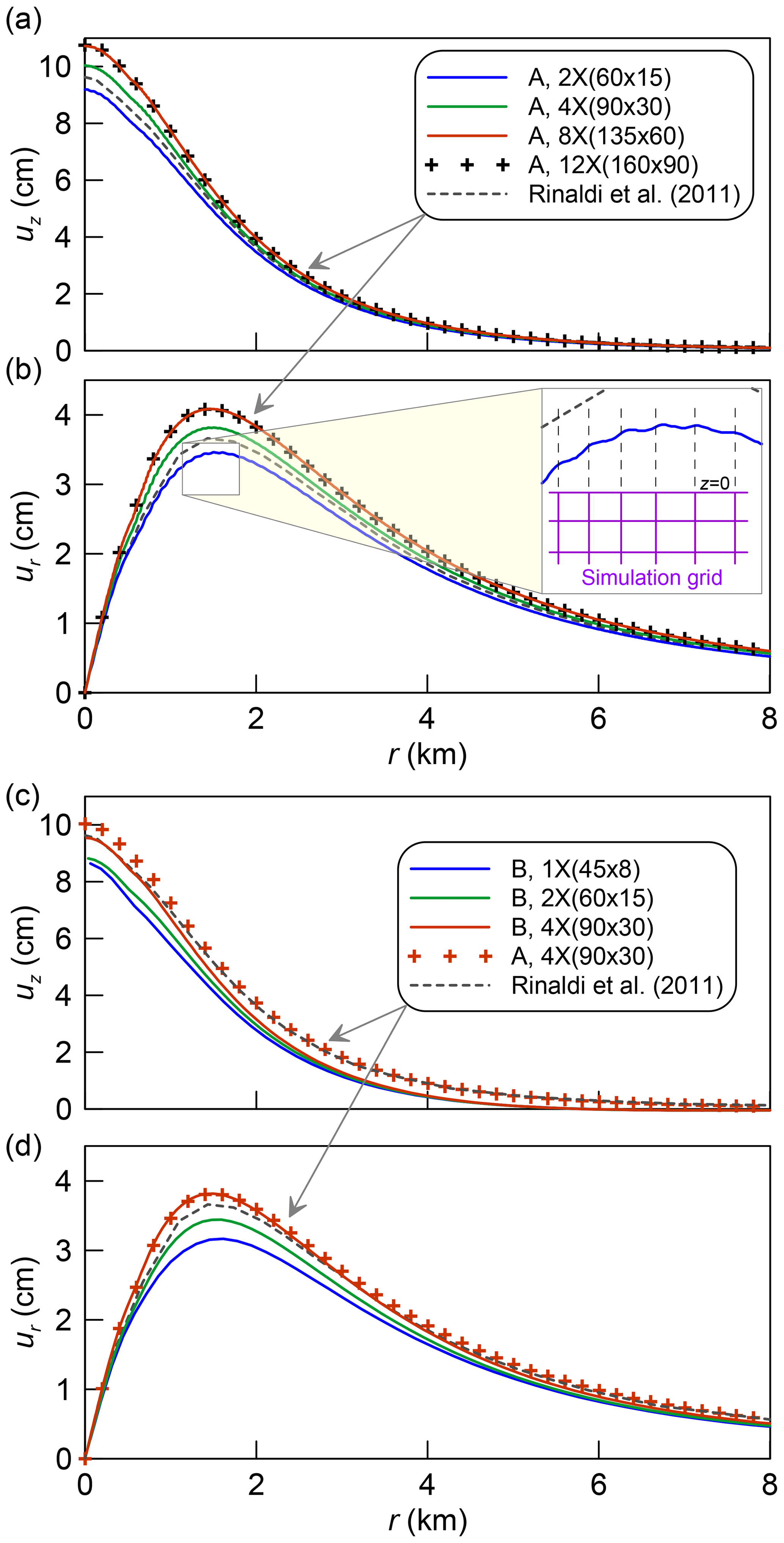
Figure 9Displacements uz (a, c) and ur (b, d) at t=20 months calculated using different methods and grids. The oscillatory behaviour of u shown in (b) is caused by the space discretisation.
4.4 Modelling ground displacement in a heterogeneous reservoir
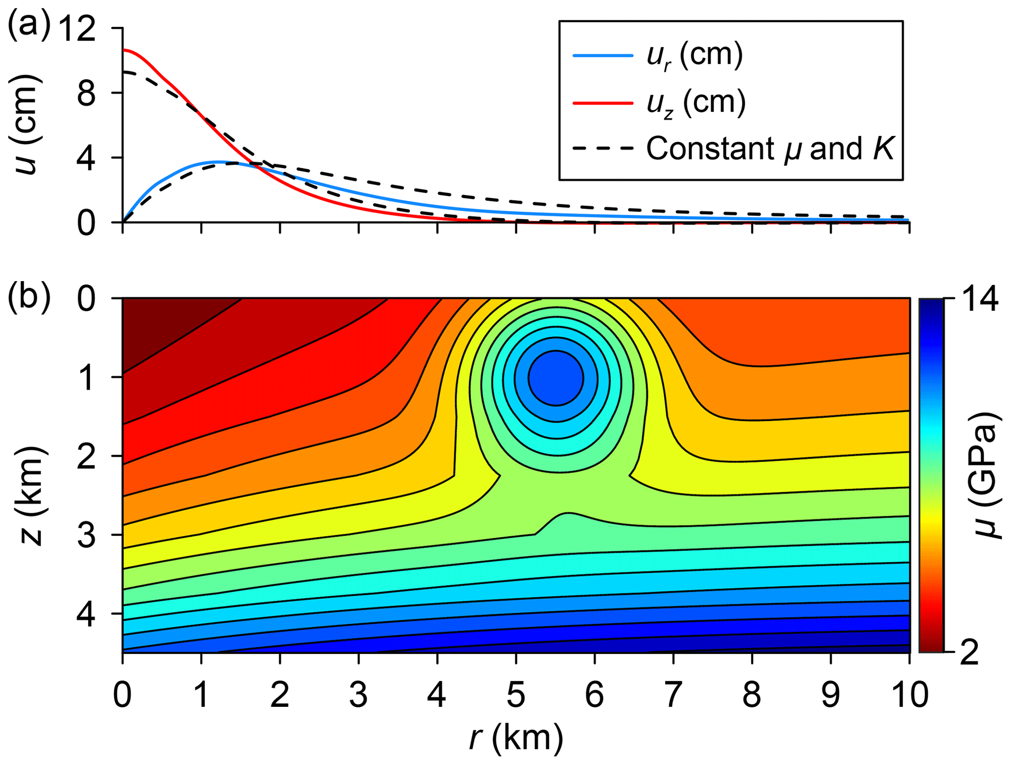
In addition to validating the geomechanical code against the semi-analytical approach, we consider another benchmark study to demonstrate the capabilities of method B for modelling hydrothermal systems with spatial heterogeneities in elastic properties of rocks. The study is identical to that described in Sect. 4.2 except for the values of μ and K. Now, the distributions of μ and K are taken to qualitatively reflect the structure of the shallow subsurface at Campi Flegrei as it is presented by Manconi et al. (2010) based on the seismic tomography study by Chiarabba and Moretti (2006). Shear modulus μ shown in Fig. 10 varies in the range of 2–14 GPa, and Poisson's ratio ν lies in the range of 0.2–0.4. The general trend is that μ rises exponentially with depth. Closer to the axis of symmetry, i.e., inside the caldera, the material is softer. A thoroidally shaped inclusion composed of much stiffer material, which models the caldera rim, is located approximately 5.5 km from the axis. Assuming that the stiffer material is also less compressible, the Poisson's ratio ν is linearly interpolated between 0.2 and 0.4 to match the minimal and maximal values of μ, respectively. The drained bulk modulus K is then calculated according to the relation
The distributions of ur and uz at z=0 calculated with the described distribution of mechanical properties do not differ much from those calculated under the assumption of a homogeneous medium (Fig. 10). The deviation from the results presented in Sect. 4.3 does not exceed 20 %. This can be explained by the synthetic nature of the benchmark, in that K is artificially constrained to enforce consistency with the range of ν without direct relation to the seismic data. Furthermore, the results reported by Rinaldi et al. (2011) and other authors were thoroughly calibrated against observations, so the effect of incorporating heterogeneities into the numerical model is not expected to be significant in this particular case.
The developed extension of MUFITS allows for the convenient built-in calculations of ground displacement and gravity changes. These calculations are performed automatically by the simulator without the involvement of any external post-processing utilities. As a consequence, the reservoir models developed and simulated with MUFITS can now be history matched to the observations of gravity changes and ground displacement. This software development, although quite straightforward, makes MUFITS closer to a universal package for modelling flows in hydrothermal systems. The developed modelling options, applied here in a study of hydrothermal activity, can also be utilised in other applications, including oil and gas extraction (Fig. 1), by employing a different fluid property module of the simulator (Afanasyev, 2015).
The simulation results also demonstrate an acceptable accuracy of the semi-empirical approach (method A) for predicting ground displacement. Given that the necessary assumptions in Sect. 2.4 are satisfied, the displacements predicted by utilising analytical solution given by Eqs. (3) and (4) are indistinguishable from those predicted by the more comprehensive approach (method B). This makes method A very attractive because it is fast and can easily deal with 3-D flows. However, if the assumptions in Sect. 2.4 are violated, then the coupling with the geomechanical code remains the only reliable approach for the ground displacement modelling. For example, the thermo-hydromechanical coupling is the only approach to assess the mechanical integrity of reservoirs consisting of the layers with significantly different poroelastic properties (e.g., sandstone layers alternating with shales) or complicated by the presence of faults. To assess the reservoir integrity, one needs to know the distribution of stresses in the entire domain, which is readily available with method B. The influence of topography, e.g., a load of volcanic edifice, on the subsurface flows and the ground displacement can be estimated only by method B. Besides the space heterogeneity, the semi-empirical method, unlike method B, does not allow for generalization to inelastic behaviour of saturated rocks, e.g., at high temperatures (>350 ∘C) that can be achieved in hydrothermal systems. The extension of MUFITS onto these cases remains a subject of further code development.
The executable of the extended version of MUFITS as well as its Reference manual can be downloaded at http://www.mufits.imec.msu.ru (Afanasyev, 2020a). The input data file for the simulator of the considered benchmark study can be downloaded at http://www.mufits.imec.msu.ru/example-cf-shallow.html (Afanasyev, 2020b). The geomechanical code can be downloaded at https://github.com/utkinis/THM2D-U (Utkin, 2020).
AA developed the modelling options for the gravity changes and ground displacement by method A. IU developed the geomechanical code (method B) and coupled it with MUFITS.
The authors declare that they have no conflict of interest.
This article is part of the special issue “European Geosciences Union General Assembly 2020, EGU Division Energy, Resources & Environment (ERE)”. It is a result of the EGU General Assembly 2020, 4–8 May 2020.
The authors acknowledge funding from the Russian Science Foundation under grant # 19-71-10051. The authors would like to thank Armando Coco and an anonymous reviewer for their extensive and constructive comments during the review of this manuscript.
This research has been supported by the Russian Science Foundation (grant no. 19-71-10051).
This paper was edited by Antonio Pio Rinaldi and reviewed by Armando Coco and one anonymous referee.
Afanasyev, A.: Hydrodynamic Modelling of Petroleum Reservoirs using Simulator MUFITS, Enrgy. Proced., 76, 427–435, https://doi.org/10.1016/j.egypro.2015.07.861, 2015. a, b
Afanasyev, A.: MUFITS Reservoir Simulation Software, available at: http://www.mufits.imec.msu.ru/, last access: 18 October 2020a. a
Afanasyev, A.: Modelling Ground Displacement and Gravity Changes, available at: http://www.mufits.imec.msu.ru/example-cf-shallow.html, last access: 18 October 2020b. a
Afanasyev, A., Costa, A., and Chiodini, G.: Investigation of hydrothermal activity at Campi Flegrei caldera using 3D numerical simulations: Extension to high temperature processes, J. Volcanol. Geoth. Res., 299, 68–77, https://doi.org/10.1016/j.jvolgeores.2015.04.004, 2015. a, b, c
Afanasyev, A., Blundy, J., Melnik, O., and Sparks, S.: Formation of magmatic brine lenses via focussed fluid-flow beneath volcanoes, Earth Planet. Sc. Lett., 486, 119–128, https://doi.org/10.1016/j.epsl.2018.01.013, 2018. a
Afanasyev, A. A.: Application of the Reservoir Simulator MUFITS for 3D Modelling of CO2 Storage in Geological Formations, Enrgy. Proced., 40, 365–374, https://doi.org/10.1016/j.egypro.2013.08.042, 2013. a
Afanasyev, A. A., Melnik, O., Porritt, L., Schumacher, J. C., and Sparks, R. S. J.: Hydrothermal alteration of kimberlite by convective flows of external water, Contrib. Mineral. Petr., 168, 1038, https://doi.org/10.1007/s00410-014-1038-y, 2014. a
Chiarabba, C. and Moretti, M.: An insight into the unrest phenomena at the Campi Flegrei caldera from Vp and Vp/Vs tomography, Terra Nova, 18, 373–379, https://doi.org/10.1111/j.1365-3121.2006.00701.x, 2006. a, b
Chiodini, G., Todesco, M., Caliro, S., Del Gaudio, C., Macedonio, G., and Russo, M.: Magma degassing as a trigger of bradyseismic events: The case of Phlegrean Fields (Italy), Geophys. Res. Lett., 30, 1434, https://doi.org/10.1029/2002GL016790, 2003. a, b, c, d
Chiodini, G., Paonita, A., Aiuppa, A., Costa, A., Caliro, S., De Martino, P., Acocella, V., and Vandemeulebrouck, J.: Magmas near the critical degassing pressure drive volcanic unrest towards a critical state, Nat. Commun., 7, 13712, https://doi.org/10.1038/ncomms13712, 2016. a
Coco, A., Gottsmann, J., Whitaker, F., Rust, A., Currenti, G., Jasim, A., and Bunney, S.: Numerical models for ground deformation and gravity changes during volcanic unrest: simulating the hydrothermal system dynamics of a restless caldera, Solid Earth, 7, 557–577, https://doi.org/10.5194/se-7-557-2016, 2016. a
Coussy, O.: Poromechanics, John Wiley & Sons, Chichester, 2004. a
Duretz, T., Räss, L., Podladchikov, Y. Y., and Schmalholz, S. M.: Resolving thermomechanical coupling in two and three dimensions: spontaneous strain localization owing to shear heating, Geophys. J. Int. 216, 365–379, https://doi.org/10.1093/gji/ggy434, 2018. a
Fanchi, J. R.: Principles of Applied Reservoir Simulation, Elsevier, Cambridge, MA, https://doi.org/10.1016/B978-0-7506-7933-6.X5000-4, 2006. a
Frankel, S. P.: Convergence Rates of Iterative Treatments of Partial Differential Equations, Mathematical Tables and Other Aids to Computation, 4, 65, https://doi.org/10.2307/2002770, 1950. a
Hayba, D. O. and Ingebritsen, S. E.: Multiphase groundwater flow near cooling plutons, J. Geophys. Res.-Sol. Ea., 102, 12235–12252, https://doi.org/10.1029/97JB00552, 1997. a
Hurwitz, S., Christiansen, L. B., and Hsieh, P. A.: Hydrothermal fluid flow and deformation in large calderas: Inferences from numerical simulations, J. Geophys. Res., 112, B02206, https://doi.org/10.1029/2006JB004689, 2007. a
Hutnak, M., Hurwitz, S., Ingebritsen, S. E., and Hsieh, P. A.: Numerical models of caldera deformation: Effects of multiphase and multicomponent hydrothermal fluid flow, J. Geophys. Res., 114, B04411, https://doi.org/10.1029/2008JB006151, 2009. a
Manconi, A., Walter, T. R., Manzo, M., Zeni, G., Tizzani, P., Sansosti, E., and Lanari, R.: On the effects of 3-D mechanical heterogeneities at Campi Flegrei caldera, southern Italy, J. Geophys. Res., 115, B08405, https://doi.org/10.1029/2009JB007099, 2010. a, b
Mindlin, R. D.: Force at a Point in the Interior of a Semi‐Infinite Solid, Physics (College. Park. Md)., 7, 195–202, https://doi.org/10.1063/1.1745385, 1936. a
Mindlin, R. D. and Cheng, D. H.: Nuclei of Strain in the Semi‐Infinite Solid, J. Appl. Phys., 21, 926–930, https://doi.org/10.1063/1.1699785, 1950. a, b
Pruess, K., Oldenburg, C., and Moridic, G.: TOUGH2 User's Guide Version 2.0, Tech. rep., Lawrence Berkeley National Laboratory, Berkeley, 1999. a
Rinaldi, A., Todesco, M., Vandemeulebrouck, J., Revil, A., and Bonafede, M.: Electrical conductivity, ground displacement, gravity changes, and gas flow at Solfatara crater (Campi Flegrei caldera, Italy): Results from numerical modeling, J. Volcanol. Geoth. Res., 207, 93–105, https://doi.org/10.1016/j.jvolgeores.2011.07.008, 2011. a, b, c, d, e, f, g, h, i, j, k
Rinaldi, A. P., Todesco, M., and Bonafede, M.: Hydrothermal instability and ground displacement at the Campi Flegrei caldera, Phys. Earth Planet. Int., 178, 155–161, https://doi.org/10.1016/j.pepi.2009.09.005, 2010. a, b, c, d
Rutqvist, J.: Status of the TOUGH-FLAC simulator and recent applications related to coupled fluid flow and crustal deformations, Comput. Geosci., 37, 739–750, https://doi.org/10.1016/j.cageo.2010.08.006, 2011. a
Räss, L., Duretz, T., and Podladchikov, Y. Y.: Resolving hydromechanical coupling in two and three dimensions: spontaneous channelling of porous fluids owing to decompaction weakening, Geophys. J. Int., 218, 1591–1616, https://doi.org/10.1093/gji/ggz239, 2019. a
Todesco, M.: Signals from the Campi Flegrei hydrothermal system: Role of a “magmatic” source of fluids, J. Geophys. Res., 114, B05201, https://doi.org/10.1029/2008JB006134, 2009. a, b, c, d
Todesco, M., Chiodini, G., and Macedonio, G.: Monitoring and modelling hydrothermal fluid emission at La Solfatara (Phlegrean Fields, Italy). An interdisciplinary approach to the study of diffuse degassing, J. Volcanol. Geoth. Res., 125, 57–79, https://doi.org/10.1016/S0377-0273(03)00089-1, 2003. a
Todesco, M., Rutqvist, J., Chiodini, G., Pruess, K., and Oldenburg, C. M.: Modeling of recent volcanic episodes at Phlegrean Fields (Italy): geochemical variations and ground deformation, Geothermics, 33, 531–547, https://doi.org/10.1016/j.geothermics.2003.08.014, 2004. a, b
Trasatti, E., Giunchi, C., and Bonafede, M.: Structural and rheological constraints on source depth and overpressure estimates at the Campi Flegrei caldera, Italy, J. Volcanol. Geoth. Res., 144, 105–118, https://doi.org/10.1016/j.jvolgeores.2004.11.019, 2005. a
Troiano, A., Di Giuseppe, M. G., Petrillo, Z., Troise, C., and De Natale, G.: Ground deformation at calderas driven by fluid injection: Modelling unrest episodes at Campi Flegrei (Italy), Geophys. J. Int., 187, 833–847, https://doi.org/10.1111/j.1365-246X.2011.05149.x, 2011. a
Utkin, I.: THM-U Software Module, GitHub, available at: https://github.com/utkinis/THM2D-U, last access: 2 May 2020. a