Layout optimization for offshore wind farms in India using the genetic algorithm technique

Wind Farm Layout Optimization Problem (WFLOP) is a critical issue when installing a large wind farm. Many studies have focused on the WFLOP but only for a limited number of turbines and idealized wind speed distributions. In this study, we apply the Genetic Algorithm (GA) to solve the WFLOP for large hypothetical offshore wind farms using real wind data. GA mimics the natural selection process observed in nature, which is the survival of the fittest. The study site is the Palk Strait, located between India and Sri Lanka. This site is a potential hotspot of offshore wind in India. A modified Jensen wake model is used to calculate the wake losses. GA is used to produce optimal layouts for four different wind farms at the specified site. We use two different optimization approaches: one where the number of turbines is kept the same as the thumb rule layout and another where the number of turbines is allowed to vary. The results show that layout optimization leads to large improvements in power generation (up to 28 %), efficiency (up to 34 %), and cost (up to 25 %) compared to the thumb rule due to the reduction in wake losses. Optimized layouts where both the number and locations of turbines are allowed to vary produce better results in terms of efficiency and cost but also leads to lower installed capacity and power generation. Wind energy is growing at an unprecedented rate in India. Easily accessible terrestrial wind resources are almost saturated, and offshore wind is the new frontier. This study can play an important role while taking the first steps towards the expansion of offshore wind in India.

1 Introduction

The Wind Farm Layout Optimization Problem (WFLOP) is a well-known problem in wind energy meteorology. WFLOP is about designing an optimal wind farm layout by finding the optimal locations for the turbines within the wind farm to reduce the wake effects and thus increase the power production (Yang et al., 2019). The simplest solution to WFLOP is the thumb rule widely acknowledged in the industry that proposes a 5–10 rotor diameter spacing along the flow direction to reduce wake effects and increase the power production by each turbine.

State-of-the-art methods to solve the WFLOP use much more complex approaches by accounting for wind speed variability, wind farm area and cost trade-offs. These methods use Calculus-based, Heuristic and Meta-Heuristic approaches. Calculus-based approaches use first and second order derivatives of the objective function to search for the optimal solution. Popular calculus-based methods include Mixed-Integer Nonlinear Programming (Donovan, 2005; Turner et al., 2014; MirHassani and Yarahmadi, 2017) and gradient-based approach (Guirguis et al., 2017; Tingey and Ning, 2017). The problem with Calculus-based approaches is they impose stringent conditions on the nature of the objective function (Herbert-Acero et al., 2014) to achieve a perfect solution. Heuristic methods use simple approaches to provide near-optimal solutions to the WFLOP. Studies with heuristic methods have used a wide range of approaches including random search (Wagner et al., 2013; Feng and Shen, 2015), harmony search (Kallioras et al., 2015), pattern search (DuPont et al., 2016), greedy heuristics (Chen et al., 2016), Monte Carlo simulation (Marmidis et al., 2008), Ant Colony Optimization (Eroglu and Seçkiner 2012), etc. The drawback of heuristic methods is the large computational time requirement. Metaheuristic methods reduce the computing time by drawing lessons from optimization processes occurring in nature (Herbert-Acero et al., 2014). Various metaheuristic methods used in WFLOP studies are Simulated Annealing (Samorani, 2013; Yang et al., 2019), Particle Swarm Optimization (Hou et al., 2016; Pillai et al., 2018), and Evolutionary Algorithm (Kusiak and Song, 2010; Song et al., 2016).

The most popular and widely used metaheuristic method is the Genetic Algorithm (GA, Herbert-Acero et al., 2014). GA is based on Darwin's theory of evolution driven by the concept of survival of the fittest. This is an iterative method where each iteration considers a set of possible optimal layouts. The best two layouts are selected and combined using genetic operators like cross-over and mutation to create another set of layouts for the next iteration. In this way, like Darwinian evolution, each iteration tends to produce better and better solutions till convergence is achieved. Perhaps the first attempt at solving WFLOP using GA was made by Mosetti et al. (1994) using 100 possible positions for the turbine placement and three hypothetical wind scenarios. A similar study was carried out by Grady et al. (2005) fixing the number of turbines in the wind farm and using the similar idealized wind scenarios. Since then, numerous studies using GA (Parada et al. 2017; Gao et al. 2015; Mayo and Daoud, 2016; Yamani Douzi Sorkhabi et al., 2016; Pillai et al., 2017; Song et al., 2017; Yin et al., 2017) have reported remarkable success in developing optimized layouts within a reasonable computing timeframe. Most of these studies limited themselves to small wind farms with 10–100 turbines and used hypothetical wind scenarios as in Grady et al. (2005).

India has one of the most ambitious renewable energy expansion programs globally, with a target of 175 GW from renewables by 2022 and 275 GW by 2027 (CEA, 2016). At the end of 2019, the installed capacities of wind and solar in India were 37 and 33 GW, respectively, while the total of all renewables was 86 GW that is more than 23 % of the total from all sources (MNRE, 2020). These figures show that despite the remarkable growth in renewables, the growth rate needs to be ramped up even higher to meet the target. Developing large offshore wind farms could be a strategy to meet this gap. India has identified an offshore wind energy potential of around 70 GW along the Gujarat coast in the west and the Tamil Nadu coast in the south-east (Dash, 2019). Apart from resource assessment, studies on offshore wind in India are minimal. The studies that have looked at offshore wind farm layouts in India have proposed rule-of-thumb layouts such as 8×7 rotor diameter spacing for a 504 MW wind farm (FOWIND, 2018) and 9.7×6.5 rotor diameter spacing for a 200 MW wind farm (FOWPI, 2018).

The objective of this study is to develop optimized layouts for massive offshore wind farms in the Palk Strait along the south-eastern coast of India operating under real-world meteorological conditions. For this purpose, we use the Genetic Algorithm technique to optimize layouts for the following scenarios:

• i.

  three wind farms along the Indian Palk Strait coastline;

• ii.

  an extremely large wind farm covering most of the Indian Exclusive Economic Zone (EEZ) in the Palk Strait.

Using the thumb rule layout of 10 rotor diameter spacing as a reference, we develop two optimized layouts for each wind farm. The first layout OPTIMAL_F uses the same number of turbines as the thumb rule and the second layout OPTIMAL_V varies the number of turbines to improve performance. The performance of the layouts is compared using efficiency and cost metrics.

2 Model description

2.1 Study site and data

The study site is the Palk Strait, a narrow 50–80 km wide waterway between the south-eastern coast of India and neighboring Sri Lanka. We used the Cross Calibrated Multi-Platform (CCMP) ocean surface wind data for our study. The CCMP data is a gridded ocean surface-vector wind analysis product produced using data from multiple sources. CCMP processing combines Version-7 RSS radiometer wind speeds, QuikSCAT and ASCAT scatterometer wind vectors, moored buoy wind data, and ERA-Interim model wind fields using a Variational Analysis Method to produce four maps daily of 0.25^∘ gridded vector winds (Atlas et al., 2011). We used wind data of 30 years (1988–2017). The wind data is available at 10 m height. The log law (Eq. 1) is used to extrapolate wind speeds to a height of 100 m as follows:

$$\begin{array}{}\text{(1)}& U_{\mathrm{100}}=U_{\mathrm{10}}\left({\displaystyle \frac{\log \left(\mathrm{100}/Z_{\mathrm{0}}\right)}{\log \left(\mathrm{10}/Z_{\mathrm{0}}\right)}}\right)\end{array}$$

where U₁₀ is the speed at 10 m height, U₁₀₀ is the speed at 100 m, and Z₀ is the surface roughness = 0.0002 for ocean surface. We used the climatology toolbox in MATLAB (Greene et al., 2019) for preparing the annual wind climatology.

The wind speed climatology from the CCMP data (Fig. 1a) confirms earlier findings (Dash, 2019; Khan et al., 2017) that the Palk Strait area is rich in wind resources and is one of the potential sites for offshore wind farms in India. The wind rose in Fig. 1b shows that the winds in this region mainly flow along the northeast (NE)–southwest (SW) directions. This phenomenon is because the area experiences the NE monsoon during the summer and SW monsoon during the winter.

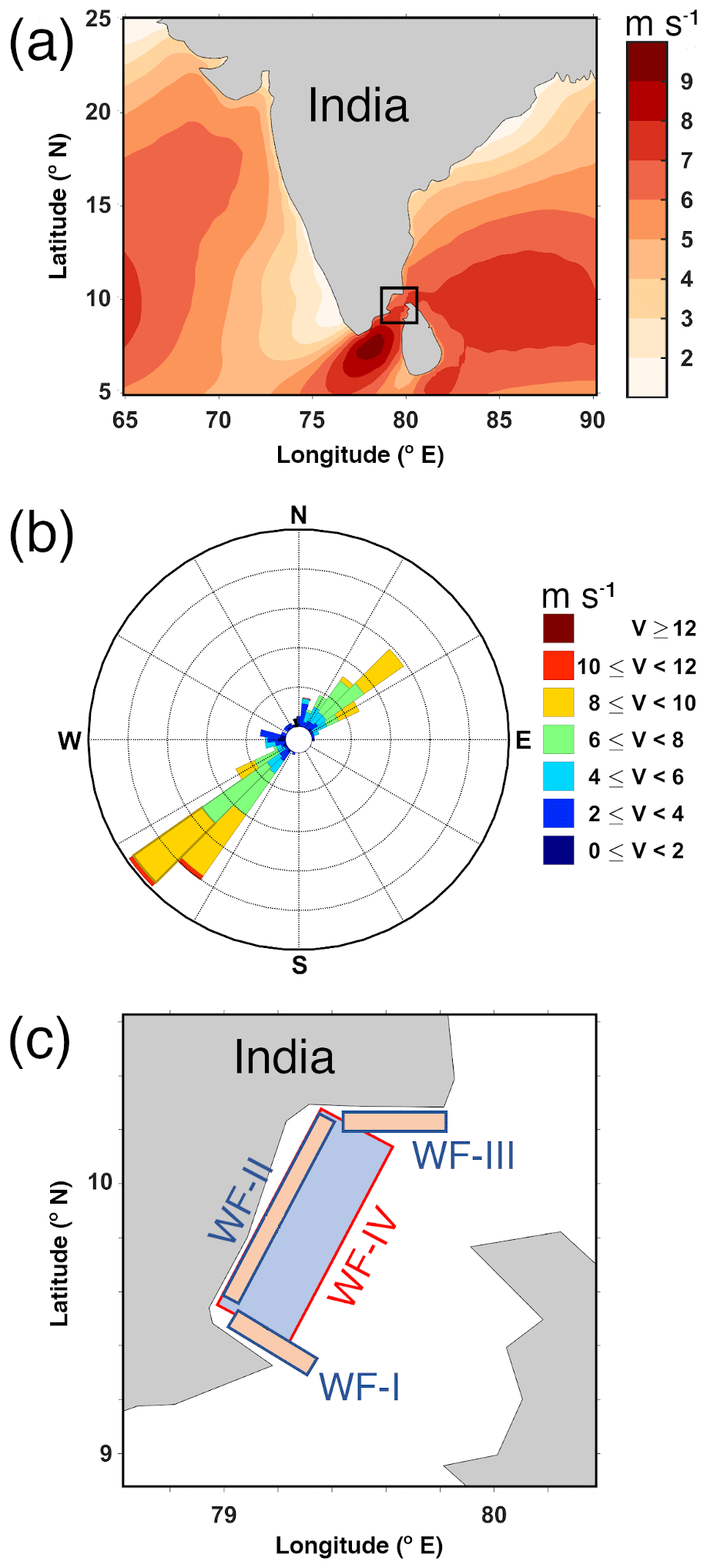
Figure 1 (a) Annual mean 100 m wind speeds from CCMP data; the black box represents the Palk Strait region. (b) The wind rose for the Palk Strait region. (c) The hypothetical wind farm scenarios considered in this study.

2.2 Windfarm scenarios

We used the following two wind farm scenarios for our study:

• i.

  A cluster of three wind farms along the Palk Strait coast depicted in Fig. 1c. The spatial dimensions of the wind farms are: WF-I: 50 D × 270 D; WF-II – 360 D × 75 D; WF-III: 50 D × 300 D; where D is the diameter of the wind turbine rotor used in this study (Table 1). These wind farms are placed quite close to the shore and, therefore, easily accessible.

• ii.

  An extremely large wind farm WF-IV, covering most of the Indian EEZ in the Palk Strait with spatial dimension: 650 D × 210 D. This wind farm perhaps sets the upper limit of the wind energy that can be harvested from this area.

Table 1 Specifications of the wind turbine used in this study.

2.3 Power model

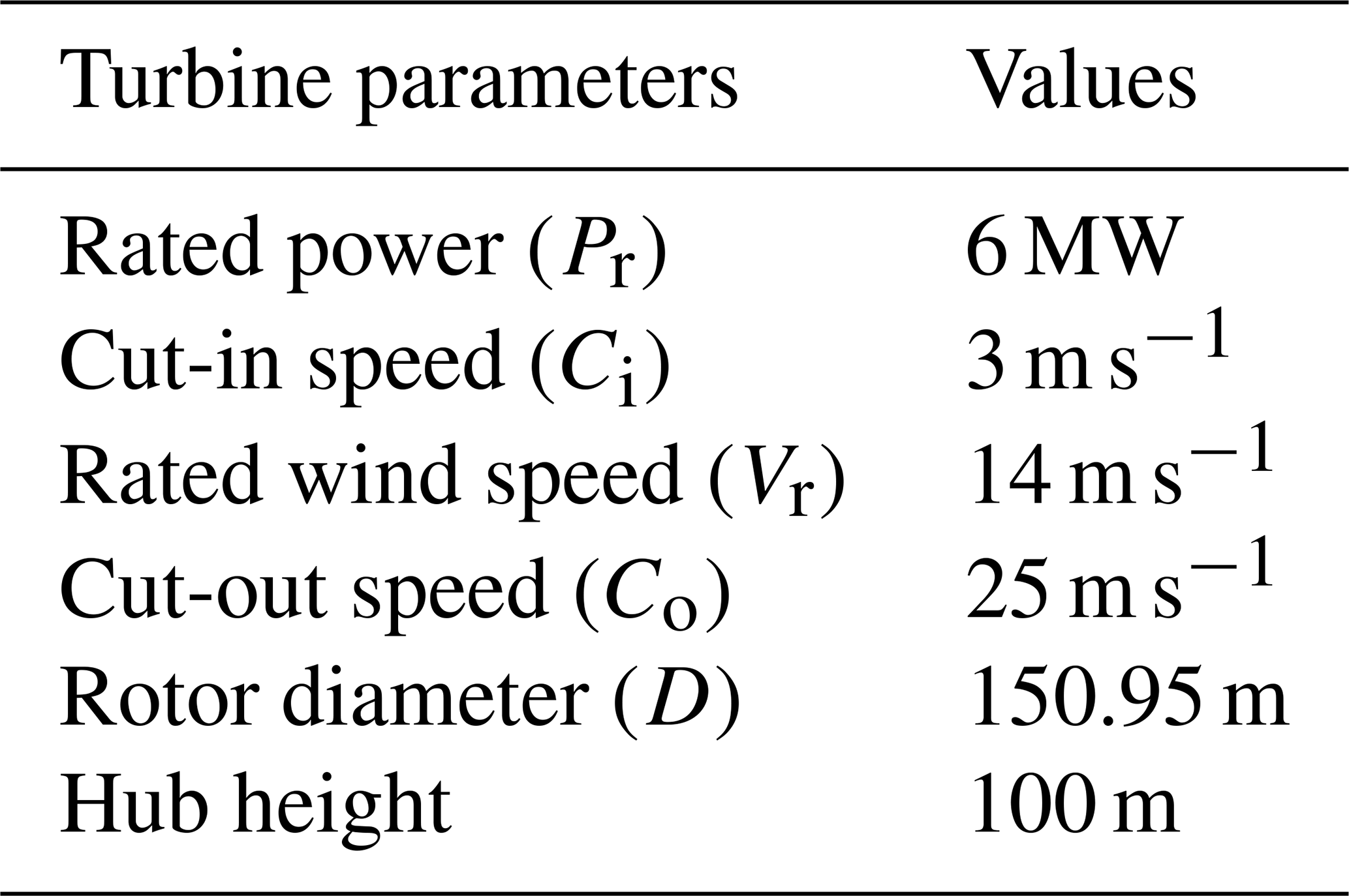
We used a hypothetical power curve shown in Fig. 2a to estimate the power generation of individual turbines. The power curve is given by the parametric model (Eq. 2) as follows:

$$\begin{array}{}\text{(2)}& P=\left\{\begin{array}{lcl}\frac{\mathrm{1}}{\mathrm{2}}\mathit{\rho }A{C}_{\mathrm{p}}{V}^{\mathrm{3}}& \forall & C_{\mathrm{i}}\le V\le V_{\mathrm{r}}\\ P_{\mathrm{r}}& \forall & V_{\mathrm{r}}\le V\le C_{\mathrm{o}}\\ \mathrm{0}& \forall & V\le C_{\mathrm{i}}\cup V\ge C_{\mathrm{o}}\end{array}\right.\end{array}$$

where P is the power generated by the turbine as a function of wind speed, V is the wind speed at the turbine hub height, A is the rotor swept area, C_i is the cut-in speed, C_o is the cut-out speed, V_r is the rated speed, and P_r is the rated power. The values of these variables are taken from a commercial wind turbine and given in Table 1. The air density ρ is constant at 1.225 kg m⁻³ that is the standard sea-level density at 288 K (ISO 2533:1975, 1975). The power coefficient C_p, a measure of the efficiency of a turbine, is the fraction of the available energy that is converted to electricity. The value of C_p is a function of the wind speed and can theoretically be as high as 0.593 that is the Betz' Limit. After sensitivity experiments, we chose a value of 0.2 that gives a realistic power curve under the constraints posed by the specifications in Table 1.

Figure 2 (a) Wind turbine power curve used in this study. (b) Jensen model schematic. (c) Wake recovery as a function of the distance from the upwind turbine for the Jensen model and the modified Jensen model used in this study.

2.4 Wake model

We used the popular Jensen model (Jensen, 1983; Herbert-Acero et al., 2014) to quantify the effects of turbine wakes on the power generation in downwind turbines. The Jensen model uses a simple mass conservation approach to estimate the velocity reduction in fully developed wakes. The model schematic is shown in Fig. 2b, and the mathematical formulation is as follows:

$$\begin{array}{}\text{(3)}& \mathrm{1}-{\displaystyle \frac{V_{\mathrm{2}}}{V_{\mathrm{1}}}}={\displaystyle \frac{\mathrm{1}-\sqrt{\mathrm{1}-C_{\mathrm{T}}}}{{\left(\mathrm{1}+\frac{k_{\mathrm{w}}\cdot x}{r}\right)}^{\mathrm{2}}}}\end{array}$$

where V₁ is the upwind speed, V₂ is the downwind speed, C_T is the thrust coefficient of the turbine, k_w is the wake decay coefficient, r is the rotor radius, and x is the distance between the turbines. The thrust coefficient is the fraction of the kinetic energy in the wind flow that is absorbed by the turbine. Even though it varies with wind speed, we used a constant value of 0.88 like many theoretical studies (Corten and Brand, 2004). Accepted values for the wake decay coefficient k_w are 0.075 for onshore sites and 0.04–0.05 for offshore sites (Katić et al., 1987). We used a value of 0.045 that is within the suggested range. The rotor radius r is obtained from Table 1, while the inter-turbine spacing x varies as per the layouts generated in the GA technique described in Sect. 2.5.

The term on the right-hand side of Eq. (3) gives the normalized wind speed deficit at a distance x downwind of a turbine (Fig. 2b). This deficit is reduced to some extent by recovery processes such as turbulent mixing of higher momentum air from outside the wake (Barthelmie et al., 2010). To simulate recovery processes, we developed an exponentially increasing wake recovery term that is closer to observations (Zhao et al., 2020) and implemented it in Eq. (3). We assumed a full wake recovery by 20 D that is a fair assumption (Højstrup, 1999). Sensitivity studies show that adding the wake recovery term leads to faster recovery of wind speeds downwind of a turbine (Fig. 2c).

For a given wind farm layout, the power model and the wake model used together allows us to simulate the total power generated by a wind farm with that particular layout.

2.5 Cost model

We estimate the cost associated with a wind farm using the cost function from Wilson et al. (2018). For simplicity, the interest on the investment is ignored. With this adjustment, the cost of a wind farm is as follows:

$$\begin{array}{}\text{(4)}& \mathrm{Cost}=\left[C_{\mathrm{t}}\cdot N+C_{\mathrm{s}}\cdot \left(N/N_{\mathrm{s}}\right)+C_{\mathrm{m}}\cdot N\right]\end{array}$$

where N is the number of turbines in the wind farm, C_t is the cost of a single turbine = 1; C_s is the cost of a single substation connecting 30 turbines = 10×C_t, N_s is the number of turbines in a substation = 30, and C_m is the maintenance cost incurred per turbine per year = 0.025×C_t. Wilson et al. (2018) had used actual costs. In contrast, we normalized the costs by the cost of a single turbine while keeping the ratios between different cost elements similar to that in Wilson et al. (2018). This approach is more flexible because the actual cost can easily be obtained by plugging in the market value of the turbine of choice in Eq. (4).

2.6 Optimization scenarios

We use two different optimization scenarios. In the first scenario (OPTIMAL_F), we keep the number of turbines the same as the number of turbines in the corresponding rule of thumb layout. In other words, this is a turbine location optimization. In the second scenario (OPTIMAL_V), both the number of turbines as well as their locations are allowed to vary.

2.7 Optimization model

There are four essential elements in the optimization problem: the design variables, the constraints, the objective/fitness function, and the optimization tool. In our study, the design variables are: number of turbines and positions of the turbines in the layout. The constraints are the area of the wind farm that is available for the turbines to occupy and the minimum distance between the turbines. The objective function is a crucial element that drives the optimization model. The goal of layout optimization is to minimize the costs per unit power produced while reducing the power loss due to wake effects. The objective function is a quantification of this goal and is given by:

$$\begin{array}{}\text{(5)}& \mathrm{OBJ}=\left[\left(w_{\mathrm{1}}\cdot {\displaystyle \frac{\mathrm{cost}}{\mathrm{energy}}}\right)+\left(w_{\mathrm{2}}\cdot {\displaystyle \frac{\mathrm{1}}{\mathrm{eff}}}\right)+\left(w_{\mathrm{3}}\cdot {\displaystyle \frac{{\mathrm{10}}^q}{N^{\mathrm{2}}}}\right)\right]\end{array}$$

where cost is the cost of the wind farm layout calculated using Eq. (4), energy is the total energy generated by the wind farm in one year estimated using Eqs. (2)) and (3), N is the number of turbines in the layout, and the Efficiency eff is the ratio of the energy generated by the wind farm with N turbines to the energy generated by N isolated turbines. The values of the coefficients w₁–w₃, and the exponent q are given at the end of this section.

The first two terms on the right hand side of Eq. (5) represent the cost and the impact of wake loss represented by the reciprocal of efficiency, respectively. It is important to note that an algorithm solely focused on increasing efficiency generates a solution where the turbines are spaced far apart, perhaps a distance of 20 D or more where there are no wake effects. Because the area of the wind farm is constrained, this solution leads to a reduction in the number of turbines, installed capacity, and power generation. The third term on the RHS is a reward term that prevents this undesirable outcome by driving the algorithm towards using a higher number of turbines while increasing efficiency. Thus, the objective of the optimization exercise is to minimize the value of OBJ by simultaneously reducing the cost, increasing efficiency, and increasing the power generation.

We use the Genetic Algorithm (GA) to solve the WFLOP in our study. The GA search procedure consists of the following steps:

• i.

  Creation of the grid: the wind farm area is discretized using a Cartesian grid with size 5 D in the dominant wind direction and 3 D in the transverse direction. Such discretization is a very commonly used approach (Mosetti et al., 1994) that is computationally more efficient than a continuous representation where the turbines are allowed to access any position within the wind farm (Charhouni et al., 2019; Kusiak and Song, 2010).

• ii.

  Creation of the initial population: the initial population consists of 34 layouts. These include two initial layouts that serve as parents. For the OPTIMAL_F scenarios, the parents are generated by placing the turbines in random locations within the wind farm area. Figure 3a(i) shows the two initial parents for the OPTIMAL_F layout for WF-I. The initial parents for the OPTIMAL_V scenarios have different patterns. The first is an extremely sparse layout where turbines are placed 20 D apart in the dominant wind direction and 12 D in the transverse direction. The second is the most densely packed layout possible with turbines at every grid point. Figure 3a(ii) shows the two initial parents for the OPTIMAL_V layout WF-I. We generate 30 layouts through crossover between the parents and 2 layouts through mutation of the parents, thus creating a population of 34 layouts. Crossover and mutation are critical parts of the GA, which resemble and replicate nature's way of creating diverse living organisms. Crossover in the current study is carried out by randomly selecting crossover points and performing uniform crossover similar to Grady et al. (2005) and González et al. (2010). Mutation is introduced by randomly picking 1 % of the grid cells and changing their state, i.e., removing a turbine if the grid cell contains a turbine or placing a turbine if the grid cell is empty.

• iii.

  Evaluation of objective function: the value of the objective function in Eq. (3) is estimated for each of these layouts.

• iv.

  Generation of the new population: a population of 34 layouts is generated using the two fittest layouts from the previous population, i.e., the 2 layouts with the lowest value of the objective function, as parents as per step ii.

• v.

  Iteration: steps iii and iv are repeated 50 000 times.

After building the wake, power, cost, and optimization models in MATLAB, hundreds of sensitivity runs were conducted to find appropriate values of the parameters in Eq. (5). Based on the results, we selected the values of the weights as follows: w₁=0.5, w₂=0.4, and w₃=0.1. The values selected for the exponent q are 4, 4.75, 4.5, and 5.75, for WF-I, WF-II, WF-III, and WF-IV, respectively. The optimization codes are run in sequential mode on an Intel i5 2.20 GHz processor take 62 and 79 s km⁻² for the OPTIMAL_F and OPTIMAL_V cases, respectively.

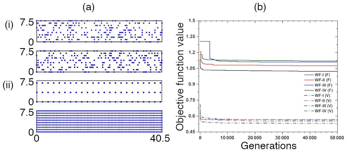
Figure 3 (a) Initial parents for the (i) OPTIMAL_F and (ii) OPTIMAL_V layouts for WF-I. (b) Evolution of the value of the objective function.

Figure 3b shows the evolution of the objective function with iterations. It can be seen that the solutions converge pretty quickly, within a few thousand iterations for all cases except WF-III. In all cases, there is very little improvement in the objective function value after 10 000 iterations. To err on the side of caution, we consider the best performing layout after the 50 000 iterations as the optimal layout.

3 Results

Figure 4 shows the different wind farms designed for the Palk Strait region. The plots show that the layouts are quite different from a typical rule of thumb regular layout. Even though the OPTIMAL_F and OPTIMAL_V layouts are different, they show similar spatial characteristics. WF-I is aligned approximately perpendicular to the prominent wind direction, while WF-II and WF-IV are approximately along the prominent wind direction. The wake effects are mostly along the prominent wind direction. Consequently, WF-I shows clustering of turbines along the length of the wind farm, but WF-II and WF-IV show clustering along the width of the wind farms. WF-III is oriented at an angle to the prominent wind direction leading to wake losses along both the length and the width. Consequently, WF-III does not show any visually discernible clustering. These patterns are observed in both the optimized layouts for each wind farm.

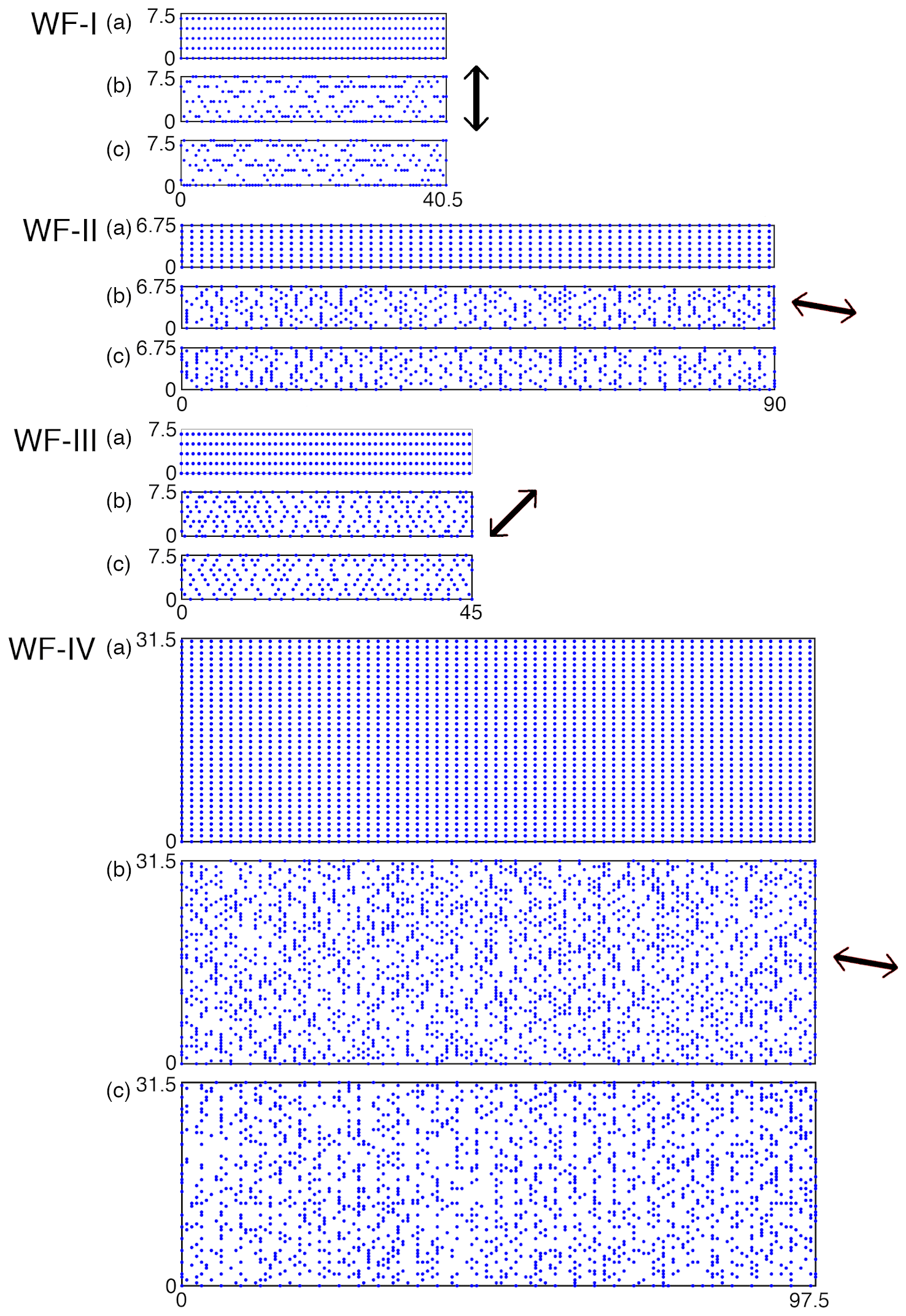
Figure 4 (a) Thumb rule, (b) OPTIMAL_F, and (c) OPTIMAL_V layouts for the four wind farms. The arrow depicts the dominant wind direction.

To quantitatively evaluate the design and performance of the optimized layouts, they are compared with the corresponding rule of thumb layouts because there is no observed data for evaluation. As mentioned earlier, in the rule of thumb layout, the turbines are placed at 10 D distance apart in the prominent wind direction and 6 D in the transverse direction. The comparison of the rule of thumb and optimal layouts given in Table 2. The results for the optimized layouts are averaged over the last 10 000 iterations. We estimate the statistical significance of the differences between the two optimized layouts using the Student's t-test.

Table 2 Comparison of design and performance metrics of the optimal layouts with the corresponding rule of thumb layouts. The metrics for the optimized layouts are averaged over the last 10 000 iterations. The numbers in the parentheses indicate percentage change with respect to the thumb rule layout.

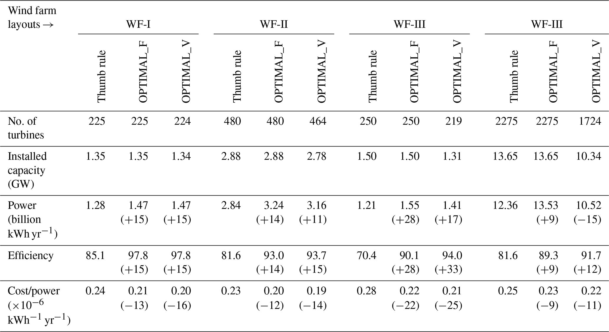
Results show that layout optimization affects all design and performance metrics in all wind farm cases. In the OPIMAL_F layouts, the number of turbines and the installed capacity remains the same as in the thumb rule but the power generation increases by 9 %–28 %. This is because layout optimization is able to reduce the wake losses and increase efficiency by 9 %–28 % compared to the thumb rule layout. Consequently, the cost/energy is also reduced by 9 %–22 %.

The OPTIMAL_V layouts also lead to improvements in performance compared to the thumb rule layouts. Efficiency is increased by 12 %–34 % and cost is reduced by 11 %–25 %. However, this optimization leads to fewer number of turbines and hence reduces the installed capacity. In spite of the reduction in installed capacity, reduced wake loss increases power generation by 11 %–17 % for WF-I, II and III. However, in WF-IV, the power generation goes down by 15 %.

OPTIMAL_V layouts perform better than the OPTIMAL_F layouts in terms of efficiency and cost. However, OPTIMAL_V layouts have fewer turbines, lower installed capacity, and generate less power than the OPTIMAL_F layouts. The differences between the two optimized layouts are statistically significant at p<0.001 but relatively small compared to their differences with the thumb rule layout.

The cluster of coastal wind farms WF-I, WF-II, and WF-III have a total installed capacity of up to 5.7 GW and produce up to 6.3 billion kWh annually. The large wind farm WF-IV can provide an approximate upper limit of wind energy availability in this region. Results show that WF-IV can have an installed capacity of up to 13.7 GW, and produce up to 13.5 billion kWh of energy annually.

4 Conclusions and discussions

This study uses the Genetic Algorithm technique to optimize layouts for hypothetical offshore wind farm scenarios in the Palk Strait off the south-eastern coast of India. The major conclusions of the study are:

• i.

  Analysis of the CCMP data confirms earlier findings that the south-east coast of India is rich in wind resources.

• ii.

  Layout optimization with the GA technique significantly affects the design and performance metrics of all wind farm scenarios. Our results show marked improvements in power generation (up to 28 %), efficiency (up to 34 %), and cost (up to 25 %) due to the reduction in wake losses.

• iii.

  Optimized layouts where both the number and locations of turbines are allowed to vary produce better results in terms of efficiency and cost. But this also leads to lower installed capacity and power generation.

Wind farm layout optimization is a popular problem. Most existing studies use small wind farms with tens to hundreds of turbines and idealized wind data. In contrast, we use large wind farms with hundreds to thousands of turbines and real-world wind data. Moreover, we conduct a comprehensive evaluation of the optimization by comparing optimized layouts with fixed and variable number of turbines against the thumb rule layout.

There is scope for methodological refinement/improvement in three different areas. First, we have used idealized functions to represent wind turbine power generation, wake losses, and wind speed recovery to generalize our results. If desired, the functions can be parameterized with turbine-specific values for parameters such as the power, thrust, and wake decay coefficients to make the results turbine-specific. Second, our idealized cost function using normalized costs can be replaced with actual market values. Third, we have parameterized the objective function using sensitivity studies. An objective approach to estimate the weights and the exponent in the objective function Eq. (5) will be a better approach even though it is computationally very expensive. Armed with these improvements, our layout optimization tool can serve as a valuable resource for the wind energy industry when expanding into the offshore regions of India or elsewhere.