Verification of a Python-based TRANsport Simulation Environment for density-driven fluid flow and coupled transport of heat and chemical species

Numerical simulation has become an inevitable tool for improving the understanding on coupled processes in the geological subsurface and its utilisation. However, most of the available open source and commercial modelling codes do not come with flexible chemical modules or simply do not offer a straight-forward way to couple third-party chemical libraries. For that reason, the simple and efficient TRANsport Simulation Environment (TRANSE) has been developed based on the Finite Difference Method in order to solve the density-driven formulation of the Darcy flow equation, coupled with the equations for transport of heat and chemical species. Simple explicit, weighted semi-implicit or fully-implicit numerical schemes are available for the solution of the system of partial differential equations, whereby the entire numerical code is composed of less than 1000 lines of Python code, only. A diffusive flux-corrected advection scheme can be employed in addition to pure upwinding to minimise numerical diffusion in advection-dominated transport problems. The objective of the present study is to verify the numerical code implementation by means of benchmarks for density-driven fluid flow and advection-dominated transport. In summary, TRANSE exhibits a very good agreement with established numerical simulation codes for the benchmarks investigated here. Consequently, its applicability to numerical density-driven flow and transport problems is proven. The main advantage of the presented numerical code is that the implementation of complex problem-specific couplings between flow, transport and chemical reactions becomes feasible without substantial investments in code development using a low-level programming language, but the easy-to-read and -learn Python programming language.

1 Introduction

Many different scientific open-source and commercial closed-source software packages are available for the simulation of fluid flow and transport processes in the geological subsurface. A comprehensive overview on the latest specific capabilities of the most popular reactive transport codes is given by Steefel et al. (2015), while many other codes exist which are also capable to handle transport of heat and chemical species (e.g., Trefry and Muffels, 2007; Flemisch et al., 2011; Koch et al., 2020; Afanasyev, 2018 among others).

Nevertheless, high flexibility is required to tackle specific (reactive) transport problems, such as those requiring the development and integration of chemical surrogate models to overcome the computational burden of chemical simulations (De Lucia et al., 2017, 2015), with a special focus on the integration of process-dependent chemical modules and/or coupling interfaces for third-party chemical modules. In this view, scientific numerical codes written in low-level programming languages (e.g., FORTRAN, C++ or C) are per se less comprehensible compared to high-level language implementations (i.e., Python), and thus limit the user who is not experienced in low-level language programming to simple code modifications.

The TRANsport Simulation Environment (TRANSE) has been developed based on the Finite Difference Method (Wang and Anderson, 1995; Clauser, 2003) to provide users familiar with high-level language programming access to the integration and coupling of arbitrary processes with thermodynamic and chemical libraries to consider chemical reactions and fluid equations of state by using Python implementations or available modules. To date, TRANSE solves the density-driven formulation of the Darcy flow equation, coupled with the equations for transport of heat and chemical species on structured grids by simple explicit, weighted semi-implicit or fully-implicit numerical schemes, and is composed of less than 1000 lines of Python (Van Rossum and Drake, 2009) code. A diffusive flux-corrected advection scheme can be employed in addition to the pure upwinding advection scheme to minimise numerical diffusion in transport problems with high Péclet numbers. Just-in-time compilation by means of the Python Numba library (Lam et al., 2015) results in computational times in the order of equivalent low-level language implementations (e.g., FORTRAN, C or C++), while CPU-based parallelisation (Anderson et al., 2017) allows for the realisation of high spatial model discretisations.

Chemical libraries, e.g., PHREEQC (Parkhurst and Appelo, 2013; Charlton and Parkhurst, 2011) and Cantera (Goodwin et al., 2017), coupled to TRANSE can be easily parallelised to increase the overall computational efficiency, whereby the latter is especially relevant as chemistry usually represents the main computational bottleneck in reactive transport simulations. Python’s Numpy library (Oliphant, 2006) is used to enable fast and efficient model parametrisation as well as simulation runtime control, whereby the Matplotlib library (Hunter, 2007) is employed for automated visualisation. More sophisticated visualisation and post-processing are achieved by using the PyEVTK library (Herrera, 2017) for exporting VTK-compatible data to the interactive visualisation software packages Mayavi (Ramachandran and Varoquaux, 2011), Paraview (Utkarsh, 2015), PyVista (Sullivan and Kaszynski, 2019) or VisIt (Childs et al., 2012).

The present study focusses on the verification of the numerical code implementation by comparison against standard numerical code benchmarks for density-driven fluid flow (Henry and Elder problems) and advective species transport (rotating cone test).

2 Materials and methods

The numerical code implementation, comprising the description of the mathematical model and solution of the resulting system of coupled partial differential equations (PDEs), as well as the benchmarks employed for the validation of the presented numerical code are discussed in the following subsections.

2.1 Numerical code implementation

The current implementation of the numerical code is designed to represent single-phase flow in porous media, conductive and convective heat transport as well as diffusive and advective species transport. Single-phase flow can be coupled with heat and/or species transport, and any external chemical reaction library that comes with a Python interface.

The Finite Difference Method is employed to solve the system of PDEs, providing the (1) pure upwind scheme and the (2) Smolarkiewicz (1983) diffusive flux-correction advection scheme for the discretisation of the advection term. The system of PDEs can be solved iteratively using a weighted explicit-implicit scheme. The Python Numba just-in-time (JIT) compiler (Lam et al., 2015) enables computational times in the order of comparable implementations in low-level languages such as FORTRAN, C or C++.

2.1.1 Mathematical model

The system of PDEs comprises the single-phase fluid flow, diffusive and advective species transport as well as conductive and convective heat transport equations, which are derived from mass and energy conservation, respectively. Single-phase fluid flow is represented by Eq. (1), with ρ_f as fluid density, ϕ as porosity, α as porous media compressibility, β as fluid compressibility, P as fluid pressure, t as time, k as permeability, μ_f as dynamic fluid viscosity, g as gravitational acceleration, z as spatial coordinate and W as source/sink term.

$$\begin{array}{}\text{(1)}& {\mathit{\rho }}_{\mathrm{f}}\left(\right(\mathrm{1}-\mathit{\varphi })\mathit{\alpha }+\mathit{\varphi }\mathit{\beta }){\displaystyle \frac{\partial P}{\partial t}}=\mathrm{\nabla }\left[{\displaystyle \frac{k{\mathit{\rho }}_{\mathrm{f}}}{{\mathit{\mu }}_{\mathrm{f}}}}(\mathrm{\nabla }P-{\mathit{\rho }}_{\mathrm{f}}g\mathrm{\nabla }z)\right]+W\end{array}$$

Equation (2) gives the diffusive and advective species transport with C as species concentration, D as diffusion-dispersion tensor, v as Darcy velocity and Q represents the source/sink mass flow rate times the source/sink species concentration. Currently, only the molecular diffusion coefficient is considered in the numerical implementation.

$$\begin{array}{}\text{(2)}& \mathit{\varphi }{\displaystyle \frac{\partial C}{\partial t}}=\mathrm{\nabla }(\mathit{\varphi }D\mathrm{\nabla }C-vC)+Q\end{array}$$

Conductive and convective transport of heat is described by Eq. (3), with c_r as porous medium specific heat capacity, ρ_r as porous medium density, c_f as fluid specific heat capacity, T as temperature, λ_r and λ_f as porous medium and fluid specific heat conductivities, respectively, and H as heat sink/source term.

$$\begin{array}{}\text{(3)}& \begin{array}{rl}{\displaystyle }\left(\right(\mathrm{1}-\mathit{\varphi })c_{\mathrm{r}}{\mathit{\rho }}_{\mathrm{r}}+& {\displaystyle }\mathit{\varphi }{c}_{\mathrm{f}}{\mathit{\rho }}_{\mathrm{f}}){\displaystyle \frac{\partial T}{\partial t}}=\\ {\displaystyle }& {\displaystyle }\mathrm{\nabla }\left[\right((\mathrm{1}-\mathit{\varphi }){\mathit{\lambda }}_{\mathrm{r}}+\mathit{\varphi }{\mathit{\lambda }}_{\mathrm{f}})\mathrm{\nabla }T-v{c}_{\mathrm{f}}{\mathit{\rho }}_{\mathrm{f}}T]+H\end{array}\end{array}$$

Two advective transport discretisation schemes are currently implemented. Equation (4) describes the pure upwind advection scheme in Einstein notation, with i referencing the node index and Δi the nodal distance. Depending on the direction of fluid flow, the concentrations or temperatures of the previous or following node are considered in the calculation of the contribution of the advective term to Eqs. (2) and (3), respectively, to maintain the positiveness of the solution.

$$\begin{array}{}\text{(4)}& {\displaystyle \frac{\partial C}{\partial t}}=-{\displaystyle \frac{\partial }{\partial i}}\left(v_{i}C\right)\cong \left\{\begin{array}{ll}-v_i\frac{C_i-C_{i-\mathrm{1}}}{\mathrm{\Delta }i},& \text{if}{v}_i>\mathrm{0}\\ -v_i\frac{C_{i+\mathrm{1}}-C_i}{\mathrm{\Delta }i},& \text{if}{v}_i<\mathrm{0}\end{array}\right.\end{array}$$

The Smolarkiewicz advection scheme is a positive-definite diffusive flux-correction scheme that requires two computational steps. First, the pure upwind advection method (cf. Eq. 4) is applied, which is then followed by the diffusive flux-correction step, reducing the implicit numerical diffusion introduced in the first step. Applying the specially defined velocity $v_i^{\mathrm{d}}$ (see Eq. 5) results in a new form of a positive-definite advection scheme with small implicit numerical diffusion. The corrective step may be optionally repeated to obtain a more accurate solution, whereby the practical application of one diffusive flux-correction step already provides sufficiently accurate results.

The main advantages of this method, compared to other flux term-correction schemes, are its small numerical diffusion and low computational costs as well as the simplicity of its practical implementation (Smolarkiewicz, 1983). Furthermore, this advection scheme requires the Courant-Friedrichs-Lewy (CFL) criterion to be fulfilled for stability. It may be also employed as a diffusive flux-correction scheme in a fully-implicit solution, when the time step size is limited by the CFL criterion.

$$\begin{array}{}\text{(5)}& \begin{array}{rl}{\displaystyle \frac{\partial C}{\partial t}}& =-{\displaystyle \frac{\partial }{\partial i}}\left(v_i^{\mathrm{d}}C\right),\\ & \text{where}{v}_i^{\mathrm{d}}\equiv \left\{\begin{array}{ll}-\frac{K_{\text{impl}}}{C}\frac{\partial C}{\partial i},& \text{if}C>\mathrm{0}\\ \mathrm{0},& \text{if}C=\mathrm{0}\end{array}\right.,\\ & \text{with}{K}_{\text{impl}}={\displaystyle \frac{\left|v_i\right|\mathrm{\Delta }i-\mathrm{\Delta }t{v}_i^{\mathrm{2}}}{\mathrm{2}}}\end{array}\end{array}$$

2.1.2 Solution of the system of partial differential equations

The Finite Difference Method is used to discretise the coupled PDEs for fluid flow as well as transport of heat and chemical species, which can be solved by explicit, semi-implicit, i.e., Crank and Nicolson (1947), and fully-implicit methods as presented by Wang and Anderson (1995) and Clauser (2003). For that purpose, the matrix-free Gauss-Seidel method is used to solve the system of PDEs with a tuned Successive Over-Relaxation (SOR) scheme (Young, 1971). whereby a Red-Black Gauss-Seidel SOR scheme is applied to parallel computations. The size of the time steps is automatically adjusted according to the following two numerical stability criteria.

For explicit time integration, the Courant-Friedrichs-Lewy criterion (Eq. 6) ensures that the numerical advection scheme remains positively definite, so that mass and energy balances are maintained during a transport time step. Even though implicit time integration is unconditionally stable for all time step sizes, Clauser (2003) recommends to apply the CFL criterion also for the implicit scheme to limit the time step size in order to avoid oscillations in coupled flow and transport simulations.

$$\begin{array}{}\text{(6)}& \text{CFL}=\text{max}\left({\displaystyle \frac{\left|v_i\right|\mathrm{\Delta }t}{\mathit{\varphi }\mathrm{\Delta }i}}\right)\le \mathrm{1.0}\end{array}$$

The Neumann criterion ensures the stability of the second-order species diffusion (Eq. 7) and heat conduction (Eq. 8) equation terms, avoiding the inversion of the respective concentration and temperature gradients.

$$\begin{array}{}\text{(7)}& {\displaystyle }{\mathit{Ne}}_{\text{S}}=\text{max}\left({\displaystyle \frac{D_i\mathrm{\Delta }t}{\mathrm{\Delta }{i}^{\mathrm{2}}}}\right)\le \mathrm{0.5}\text{(8)}& {\displaystyle }\begin{array}{rl}{\mathit{Ne}}_{\text{H}}& =\text{max}\left({\displaystyle \frac{\mathit{\gamma }\mathrm{\Delta }t}{\mathrm{\Delta }{i}^{\mathrm{2}}}}\right)\le \mathrm{0.5},\\ & \text{with }\mathit{\gamma }={\displaystyle \frac{(\mathrm{1}-\mathit{\varphi }){\mathit{\lambda }}_{\mathrm{r}}+\mathit{\varphi }{\mathit{\lambda }}_{\mathrm{f}}}{(\mathrm{1}-\mathit{\varphi }){\mathit{\rho }}_{\mathrm{r}}{c}_{\mathrm{r}}+\mathit{\varphi }{\mathit{\rho }}_{\mathrm{f}}{c}_{\mathrm{f}}}}\end{array}\end{array}$$

Together with the two aforementioned numerical stability criteria, the Péclet number is provided to the user as runtime information to give a measure of the strength of advection relative to diffusion (Eq. 8) or conduction relative to convection (Eq. 9). Péclet numbers of Pe_S≤2 and Pe_H≤2 guarantee that oscillations do not arise in a transport simulation with explicit time integration.

$$\begin{array}{}\text{(9)}& {\displaystyle }{\text{Pe}}_{\text{S}}=\text{max}\left({\displaystyle \frac{\left|v_i\right|\mathrm{\Delta }i}{D_i}}\right)\le \mathrm{2.0}\text{(10)}& {\displaystyle }{\text{Pe}}_{\text{H}}=\text{max}\left({\displaystyle \frac{\left|v_i\right|{\mathit{\rho }}_{\mathrm{f}}{c}_{\mathrm{f}}\mathrm{\Delta }i}{\mathit{\lambda }}}\right)\le \mathrm{2.0}\end{array}$$

2.1.3 Coupling of fluid flow with the transport of species and heat

Fluid flow and transport of species and heat may be coupled by different coupling parameters in TRANSE, so that the initially linear system of PDEs becomes non-linear as soon as it depends on the feedback of fluid density, viscosity and compressibility from the change in species concentrations and/or temperature due to occurring transport processes. On the other hand, heat transport is coupled to fluid flow by the Darcy velocity in the advection term, which is derived from the pressure gradient in addition to the pressure and temperature dependency of the fluid parameters density, thermal conductivity and specific heat capacity. Similarly, species transport is coupled to fluid flow by the Darcy velocity in the advection term and concentration-dependent density changes of the fluid (i.e., due to salt dissolution).

Further, porosity and permeability changes resulting from the consideration of chemical reactions generate a direct feedback to the fluid flow equation. Temperature and pressure-dependent porous media properties (compressibility, specific heat conductivity and heat capacity) may further contribute to the aforementioned non-linearity. In the present implementation, fluid and porous media parameters are updated in the following time step, so that the process coupling strength is eventually determined by the modeller's choice of the time step size.

2.2 Definition of numerical code validation benchmarks

Two popular benchmarks for density-driven fluid flow and a benchmark for the advection term at infinite Péclet numbers are discussed in the following to demonstrate the validity of the numerical code implementation.

2.2.1 Henry problem

The Henry problem considers saltwater intrusion into a freshwater aquifer, whereby a semi-analytical method has been applied for its solution as discussed in Henry (1964). The aquifer model used for the numerical simulation of the Henry problem is illustrated in Fig. 1, initially saturated with freshwater (C=0 kg m⁻³). Impermeable boundary conditions are assigned to the top and bottom boundaries, while hydrostatic pressure with a normalised salt concentration of C =1 kg m⁻³ are set at the right boundary (seaside) by means of a Dirichlet boundary condition. A Neumann flow boundary condition with a prescribed constant flux and a Dirichlet boundary condition with a constant salt concentration of C=0 kg m⁻³ are applied at the left model boundary.

Figure 1 Model domain and boundary conditions applied to the Henry (1964) problem for numerical code validation.

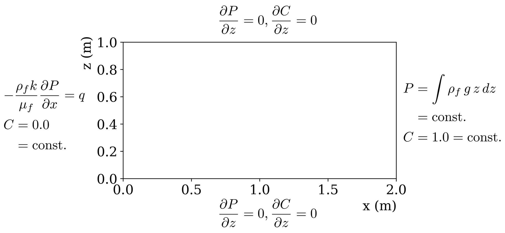
The model parametrisation used for the Henry problem is given in Table 1. The total simulation time is six days to ensure that steady-state fluid flow is achieved for the envisaged model validation as in Clauser (2003), even though Kolditz et al. (1998) report that they reach steady-state conditions already at a simulation time of 3 h. Time step sizes are determined automatically by means of the Neumann and Courant-Friedrichs-Lewy stability criteria and the system of coupled PDEs is solved in a fully implicit manner.

Table 1 Henry problem model parameters adapted from Kolditz et al. (1998).

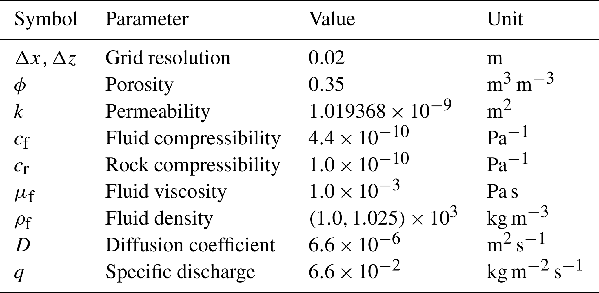
The change in fluid density ρ_f is calculated using Eq. (11) with C as normalised salt concentration, so that ρ_f may vary between 1000 and 1025 kg m⁻³. Fluid viscosity and compressibility remain constant according to the problem definition.

$$\begin{array}{}\text{(11)}& {\mathit{\rho }}_{\mathrm{f}}=(\mathrm{1000}+C\times \mathrm{25}){\text{kg\hspace{0.17em}m}}^{-\mathrm{3}}\end{array}$$

2.2.2 Elder problem

The Elder problem is a benchmark for testing free convection processes, whereby fluid flow is purely driven by differences in fluid density. In this context, Elder (1966, 1967) discusses experimental and numerical studies on thermal convection initiated by partially heating the bottom of a porous layer. The initial experimental design employed the Hele-Shaw cell for that purpose in order to verify a finite difference model that Elder used for numerical analysis of thermally-driven convection. Kolditz et al. (1998) and other authors suggest to use the Elder problem as thermal analogue for saltwater intrusion by density-driven convection. Since a characteristic salinity pattern evolves during the experiment and numerical simulations, the Elder problem is also addressed as 'fingering' problem.

The boundary conditions of the Elder problem are presented in Fig. 2, whereby the model representation here and in the following is based on the half domain due to the presence of a vertical model symmetry axis at x=300 m. All boundary conditions are closed for fluid flow, except for the upper-most left element, which is represented by a Dirichlet boundary condition (constant pressure) to compensate the changes in fluid density due to salt dissolution in the model domain (Clauser, 2003). Constant normalised salt concentrations are prescribed by Dirichlet boundary conditions at $\mathrm{0}\mathrm{m}\le x\le \mathrm{300}$ m and z=0 m with C=0 kg m⁻³ as well as at $\mathrm{150}\mathrm{m}\le x\le \mathrm{300}$ m and z=150 m with C=1 kg m⁻³. The initial salt concentration is C=0 kg m⁻³ and the initial pressure is hydrostatic, whereby fluid density is derived from Eq. (12), allowing for a density variation between 1000 and 1200 kg m⁻³. Fluid viscosity and compressibility remain constant in the present benchmark.

Figure 2 Model domain and boundary conditions applied to the Elder problem for numerical code validation.

$$\begin{array}{}\text{(12)}& {\mathit{\rho }}_{\mathrm{f}}=(\mathrm{1000}+C\times \mathrm{200}){\mathrm{kg}\mathrm{m}}^{-\mathrm{3}}\end{array}$$

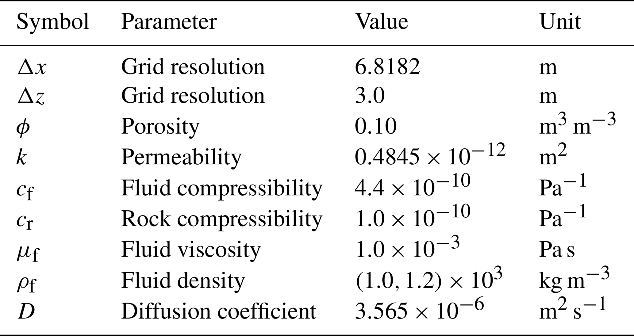
The model parametrisation used for the Elder problem is given in Table 2. Total simulation time is 20 years, with the maximum feasible time step sizes being automatically determined by the Neumann and Courant-Friedrichs-Lewy stability criteria for the diffusion and advection term, respectively. The system of PDEs for fluid flow is solved in a fully-implicit manner, while species transport is computed fully explicit.

Table 2 Elder problem model parameters adapted from Kolditz et al. (1998).

2.2.3 Rotating cone test

The rotating cone test introduced by Smolarkiewicz (1983) represents a standard benchmark to assess the numerical diffusion of an advection scheme. Figure 3 shows the initial location of the tracer distribution, represented by a cone with a peak concentration of C=3.87 kg m⁻³ and diameter of 30 m. The cone is rotated six times around the model centre (x=50 m, y=50 m) at a constant angular velocity in counter-clockwise direction. It has to be noted that the Péclet number equals infinity, since the molecular diffusion coefficient is set to zero in the present benchmark example. Dirichlet boundary conditions are applied at all four model boundaries with C=0 kg m⁻³ and the total simulation time is 376.8 s at a time step size of Δt=0.1 s.

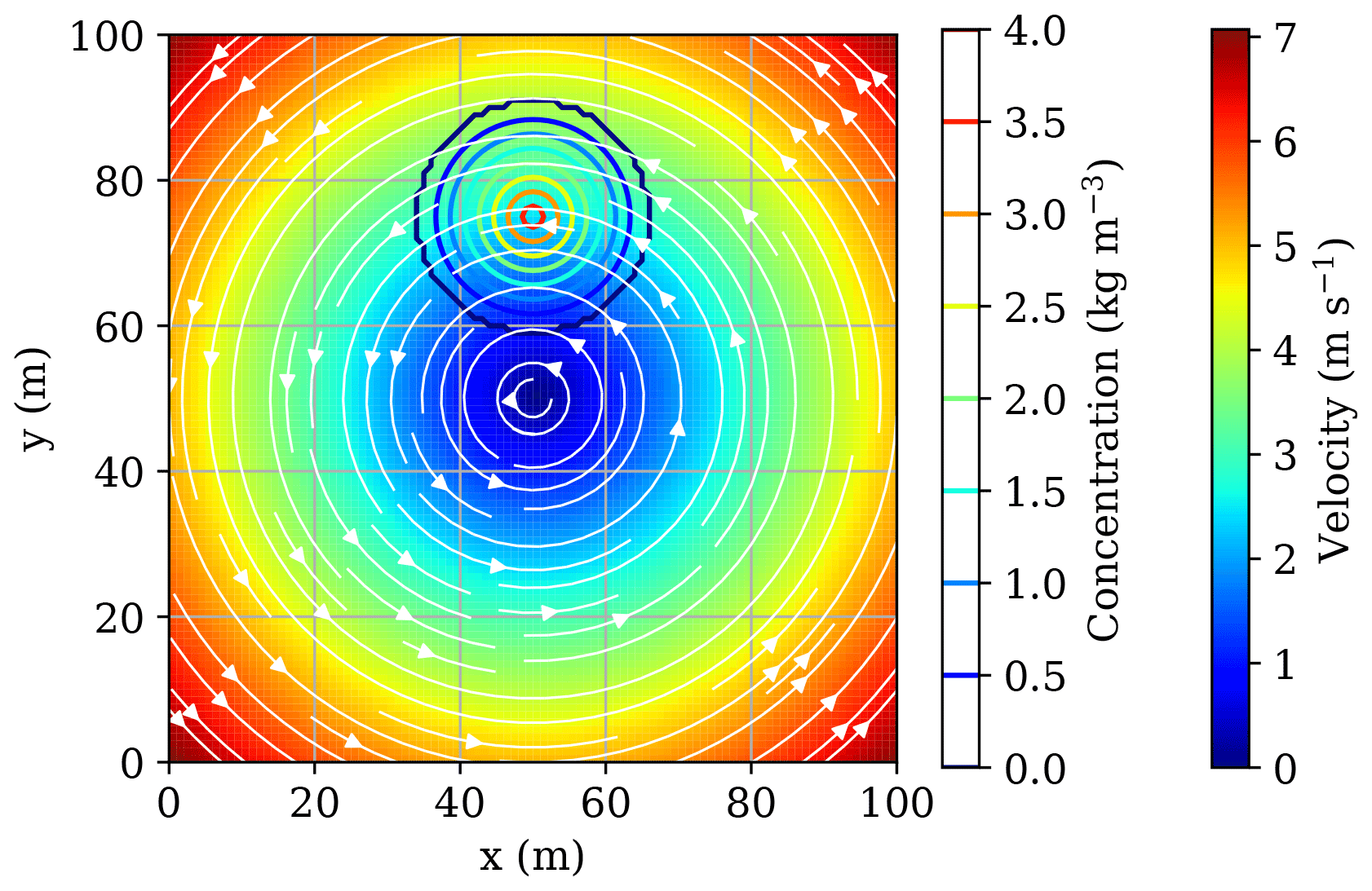
Figure 3 Spatial model dimensions, initial tracer concentration and prescribed spatial velocity field used for the rotating cone test. Contour lines show the initial shape with a maximum of C=3.87 kg m⁻³ and the exact location of the 30 m diameter cone, while the filled contours and streamlines illustrate the prescribed spatial velocity distribution.

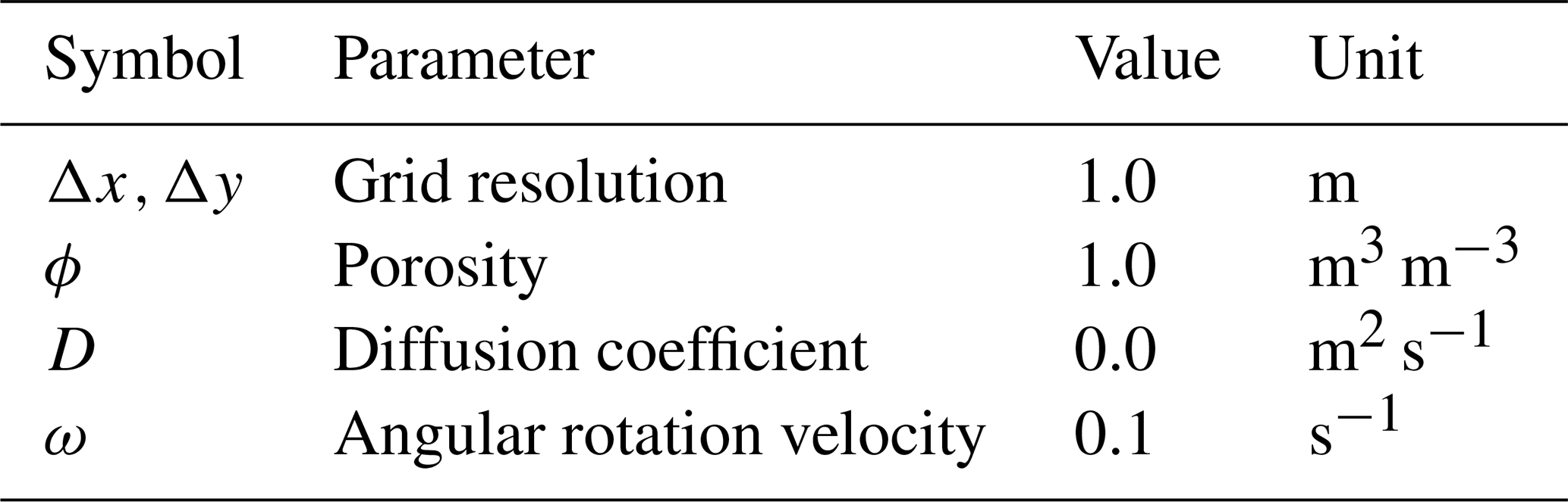
Table 3 summarises the model parametrisation employed for the rotating cone test. Fluid flow is not calculated, since angular velocity, and thus a velocity field is prescribed. A fully-explicit scheme is chosen for the solution of the resulting system of PDEs, considering the Courant-Friedrichs-Lewy and Neumann criteria to guarantee numerical stability.

Table 3 Rotating cone test parameters adapted from Smolarkiewicz (1983).

3 Results and discussion

The following subsections comprise the presentation of the simulation results and their discussion in the context of numerical code validation.

3.1 Henry problem

At steady-state fluid flow conditions, seawater has intruded via the right model boundary into the model domain. Consequently, the highest densities are found in this area, driving the saltwater intrusion. On the other hand, the constant freshwater influx at the left model boundary introduces another driving force into the model aquifer. Eventually, the initially density-driven velocity directions are reversed into the right direction, so that the less dense fluid leaves the model domain via the upper right model boundary, while the denser high-saline fluid moves towards the left model boundary below the freshwater.

The simulation results for the Henry problem are compared against those produced by Kolditz et al. (1998) by means of the FEFLOW and ROCKFLOW numerical simulators as well as those presented by Clauser (2003) using the SHEMAT numerical simulator, since the results of the Henry (1964) semi-analytical solution cannot be reproduced by any numerical code (Ségol, 1994). Please refer to Kolditz et al. (1998) for the full discussion of this Henry problem “mystery”.

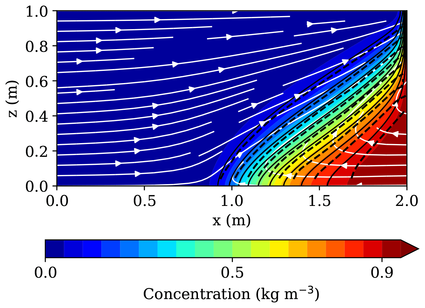
Figure 4 shows the comparison of the 0.25, 0.5 and 0.75 isochlors produced by ROCKFLOW, FEFLOW and TRANSE. All three isochlors are in very good agreement, except for minor deviations at the lower and right model boundaries. This is very likely accountable to the graphical representation of salt concentrations resulting from the Finite Element Method used for spatial discretisation in the case of the ROCKFLOW and FEFLOW simulators. It is obvious that salt concentrations cannot be zero at x=2.0 m and $\mathrm{0.8}\le z\le \mathrm{1.0}$ m, since a Dirichlet boundary condition with C=1.0 kg m⁻³ has been assigned to the right model boundary. A similar visualisation effect is expected to occur at the lower model boundary.

Figure 4 Comparison of TRANSE simulation results for the Henry problem (solid lines and contours) against 0.25, 0.5 and 0.75 isochlors computed with FEFLOW and ROCKFLOW (dashed) by Kolditz et al. (1998). White streamlines illustrate the spatial velocity field.

The comparison against the simulation results produced with the SHEMAT simulator (Clauser, 2003) is plotted in Fig. 5. While both 0.9 isochlors show a notable deviation, the agreement between both simulation results improves with the decrease in salt concentration, eventually showing a good agreement from the 0.7 isochlor on. The main reason for the deviation between the SHEMAT and TRANSE isochlors at high salt concentrations is likely the fact that the SHEMAT simulation has been undertaken using the Il'in flux blending scheme (Clauser, 2003), which introduces less numerical diffusion than the pure upwind scheme used for the TRANSE simulation. Further, the choice of fluid compressibility made for the SHEMAT simulations is one order in magnitude higher than that defined for the Henry problem by Kolditz et al. (1998), and actually also one order in magnitude higher than that of pure water at the given pressure and temperature conditions. As for the visualisation issues discussed for the ROCKFLOW and FEFLOW simulation results, interpolation errors are also observed in the SHEMAT result visualisation at the two relevant model boundaries.

Figure 5 Comparison of TRANSE simulation results for the Henry problem (solid lines and contours) against isochlors computed with SHEMAT (dashed) by Clauser (2003). White streamlines illustrate the spatial velocity field.

It has to be noted that the general deviation between the simulated isochlors in the Henry problem strongly depends on the chosen advection scheme. Voss and Souza (1987) and Kolditz et al. (1998) show that modellers using different numerical simulation codes produced deviations of the 0.5 isochlor of up to 0.1 m in x-direction at the bottom model boundary. On the contrary, the 0.5 isochlor produced by TRANSE is in very good agreement with the three other simulators employed for model comparison in the present study.

3.2 Elder problem

As for the Henry problem, an exact solution for the Elder problem is not available. Consequently, the comparison to the results published by authors of other numerical simulation studies is required for code validation. To avoid the impact of discretisation effects, grid sizes used here are identical with those applied in the simulation studies discussed by Clauser (2003) and Kolditz et al. (1998). However, only the simulation results produced with the SHEMAT simulator are used here for model comparison, since both numerical codes make use of the Finite Difference Method. Further, Clauser (2003) demonstrated that the SHEMAT results are in good agreement with those presented by Voss and Souza (1987) and Kolditz et al. (1998).

Figure 6 shows the simulation results for the Elder problem at simulation times of 4, 10, 15 and 20 years, whereby the dashed lines represent the 0.2 and 0.6 isochlors resulting from the SHEMAT simulations. The isochlors at a simulation time of four years show a very good agreement, except for some minor deviations in the upper central part of the established fingering. This good agreement is also observed at a simulation time of 10 years, whereby the SHEMAT 0.6 isochlor has already migrated about 25 m farther downwards compared to the TRANSE one. Nevertheless, the 0.2 isochlors are in very good agreement at that time.

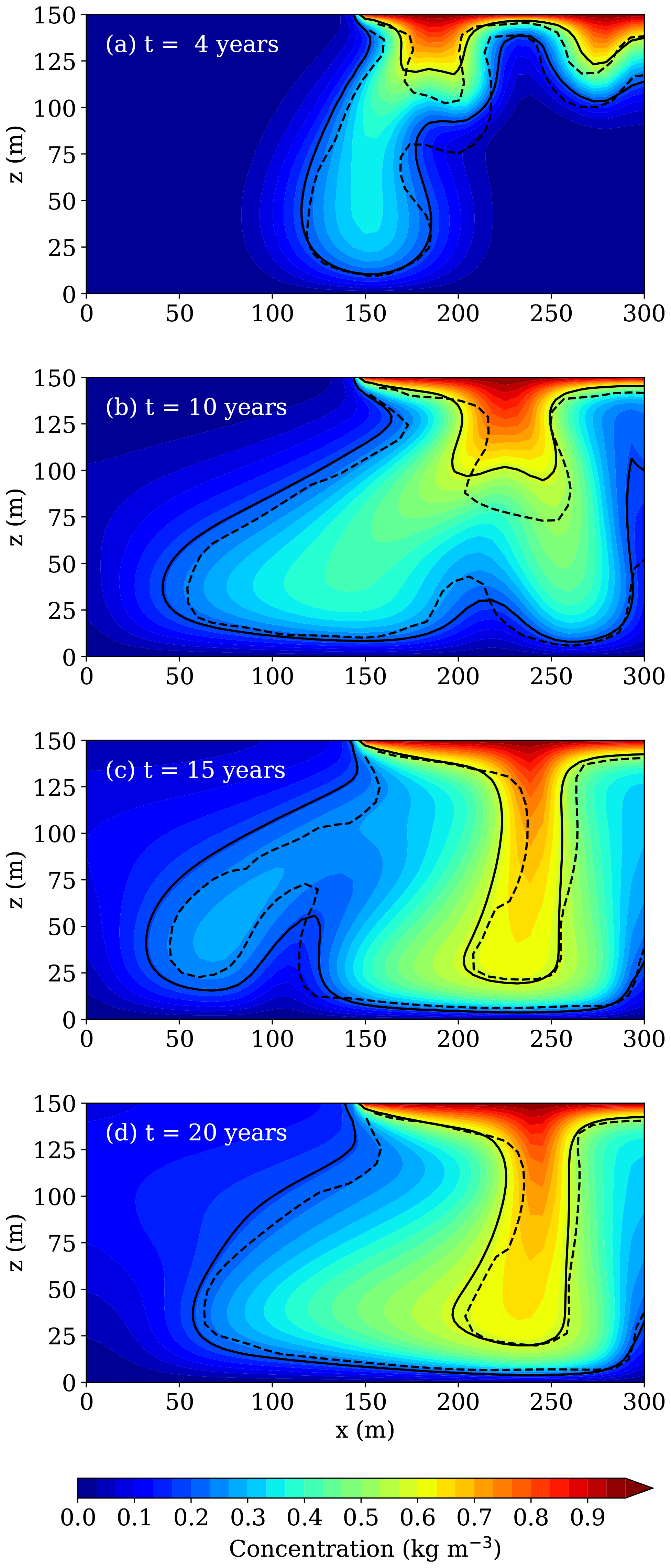
Figure 6 Comparison of the simulation results for the Elder problem using the upwind advection scheme (solid lines and contours) against SHEMAT's Smolarkiewicz advection scheme implementation results (dashed lines) for the 0.2 and 0.6 isochlors at simulation times of (a) 4 years, (b) 10 years, (c) 15 years and (d) 20 years.

After 15 years of simulation, both isochlors are in very good agreement, exhibiting only minor deviations for the 0.2 isochlors. It is important to note that the 0.2 shows the development of an additional finger in the left part of the model domain, what is especially characteristic for higher-order advection schemes, such as the Smolarkiewicz scheme that has been used for the SHEMAT simulation. However, the TRANSE simulation results plotted in Fig. 6 are obtained using the pure upwind advection scheme. At the end of the simulation time of 20 years, both isochlors are in almost perfect agreement.

Clauser (2003) demonstrates that higher-order advection schemes usually produce significant differences in the Elder problem results, compared to the first-order pure upwind advection scheme. While higher-order advection schemes produce four symmetric advection cells and upward flow in the centre of the model domain, the pure upwind scheme yields only two symmetric advection cells with downward flow in the model centre. Clauser (2003) identifies the relatively high numerical diffusion of the pure upwind advection scheme as one of the major reasons for the aforementioned differences.

Interestingly, the upwind scheme implementation in TRANSE exhibits almost identical results compared to the Smolarkiewicz scheme implementation in SHEMAT, which provides comparable results to those produced by SHEMAT's Il'in scheme implementation for the Elder problem (please refer to Clauser, 2003 for more details). After studying the SHEMAT model input data in more detail, the author of the present study expects the good agreement despite of the different advection schemes to result from the fact that the SHEMAT Elder problem model is using a non-zero longitudinal dispersion coefficient in addition to the upwinding of density used in the TRANSE flow equation implementation.

In summary, the modelling results on the Elder problem produced in the present study demonstrate TRANSE is fully capable of simulating density-driven problems at a quality level similar to that of already established numerical simulation codes.

3.3 Rotating cone benchmark

The analytical solution for the rotating cone test is straight-forward: the shape of the prescribed cone and the maximum concentration of 3.87 kg m⁻³ have to be preserved after any number of rotations for a purely advective problem. Numerical diffusion is responsible for any changes in its shape and maximum concentration.

Figure 7 shows the initial cone shape and location at the start of the simulation with a diameter of 30 m and maximum concentration of 3.87 kg m⁻³ at x=50 m and y=75 m. A diffusive flux-corrected scheme should preserve the cone shape after six full rotations (12π) following Smolarkiewicz (1983).

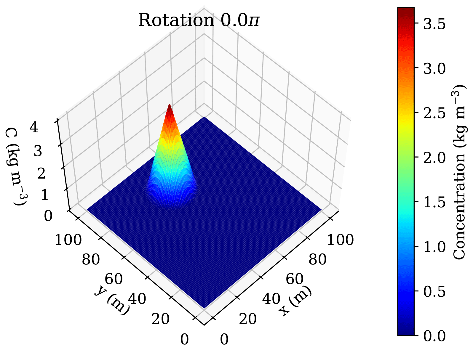
Figure 7 Initial cone shape and location at the beginning of the rotating cone test with a diameter of 30 m and maximum tracer concentration of 3.87 kg m⁻³ at x=50 m and y=75 m.

The tracer concentration after six full rotations in the rotating cone test with the pure upwind advection scheme is plotted in Fig. 8. It is obvious that the numerical diffusion accompanying the pure upwind advection scheme reduces the initial concentration by more than one order in magnitude to C=0.278 m kg⁻³ (7.2 % of the initial maximum concentration) in addition to a substantial flattening of the initial cone shape at the given infinite Péclet number. During the rotational movement, tracer is transported out of the model domain via the open boundaries by diffusion and advection. As a consequence, the upwind advection scheme is limited to problems with slow advection and moderate gradients of temperature and/or concentration. This becomes especially relevant, if chemical reactions of multiple species may introduce strong artefacts (Clauser, 2003).

Figure 9 shows the cone shape and its maximum concentration of C=3.718 kg m⁻³ (96.1 % of the initial maximum concentration) after six full rotations by means of the Smolarkiewicz advection scheme. These results are in excellent agreement with the data published by Smolarkiewicz (1983), but show a slight deviation to the SHEMAT simulation results, which exhibit a 6.45 % tracer conservation for the pure upwind advection, a 7.0 % tracer conservation for the Il'in flux blending and a 93.0 % tracer conservation for the Smolarkiewicz scheme, only. The main reason for these slight differences to the TRANSE simulation results may be accounted to the non-zero diffusion and dispersion coefficients used in the SHEMAT simulations, probably to stabilise the numerical solution procedure.

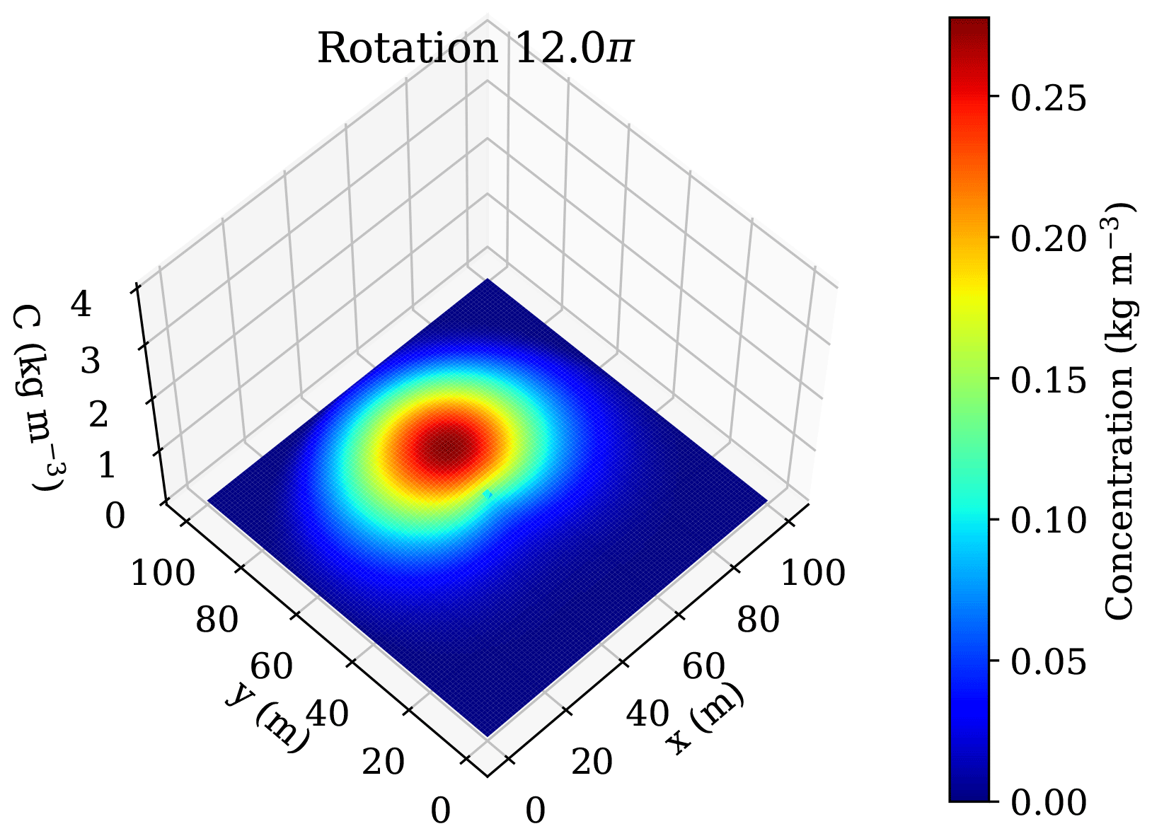
Figure 8 Cone shape and maximum tracer concentration (C=0.278 kg m⁻³) after six full rotations for the pure upwind advection scheme, which introduces substantial numerical diffusion, resulting in the preservation of only about 7 % of the maximum initial concentration.

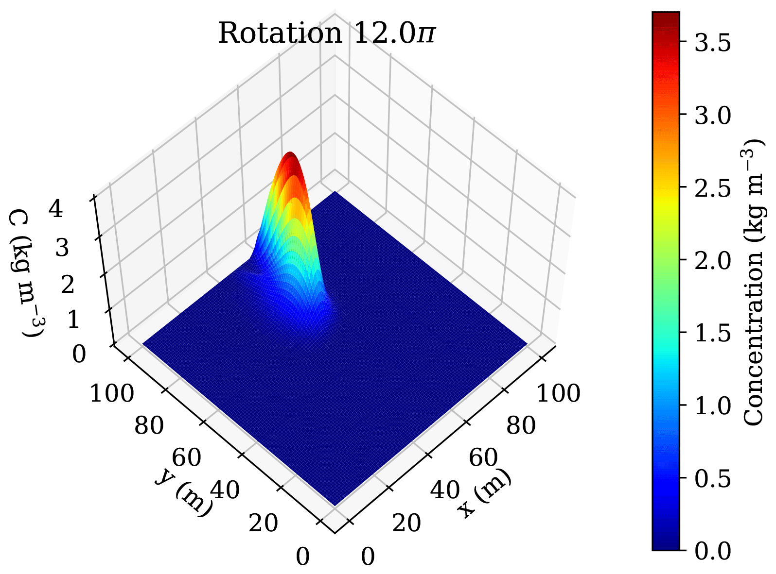
Figure 9 Cone shape and maximum tracer concentration (C=3.718 kg m⁻³) after six full rotations for the Smolarkiewicz advection scheme, which preserves more than 96 % of the initial maximum tracer concentration.

An obvious disadvantage of the Smolarkiewicz scheme is the deformation of the cone. Nevertheless, it may become acceptable given the preservation of the maximum tracer concentration. The additional computational demand of the Smolarkiewicz scheme is rather negligible, since it may also reduce the actually required iterations for the solution of the species and/or heat transport equations by the reduction of numerical diffusion. According to Clauser (2003), it is best-suited for problems where sharp concentration fronts are advected through the model domain or if the chemical equilibrium of reacting species strongly depends on the background concentration of reacting species.

4 Summary and conclusions

The TRANsport Simulation Environment has been implemented to overcome limitations of other numerical simulation codes, which in general do not provide straight-forward coupling interfaces for third-party chemical libraries or are limited by their chemical module implementations. TRANSE is based on the Finite Difference Method, whereby non-linearity is introduced by the different coupling parameters between fluid flow as well as transport of chemical species and heat to the system of PDEs. Application of just-in-time compilers ensures that the Python code implementation, which uses a high-level programming language that is relatively easy to learn and read, provides an equivalent computational performance as low-level programming languages, such as FORTRAN, C and C++, widely applied in numerical code development. CPU-based parallelisation allows for further speed-up of the numerical code implementation, enabling large-scale numerical simulations. Straight-forward conversion of Python Numpy arrays into binary VTK data supports the numerical simulation result visualisation in any VTK-compatible software package.

The present study uses three selected benchmarks for density-driven fluid flow and advection-dominated species transport, respectively, to demonstrate the general validity of the implemented numerical code. The obtained results for the Henry and Elder problems as well as the rotating cone test are in very good agreement with those produced by other accepted numerical codes. Further benchmarks that are not discussed in the scope of this manuscript have been successfully undertaken, including the Theis problem (Theis, 1935) and two hydrothermal convection problems with temperature-dependent fluid densities and viscosities discussed in Kolditz et al. (2018). The results presented in this study demonstrate that TRANSE is generally capable to handle density-driven fluid flow problems.

Especially advection-dominated species transport problems may suffer from numerical diffusion, if sharp reaction fronts occur or chemical reactions depend on the background concentrations of other reactive species (Clauser, 2003). Consequently, the implemented Smolarkiewicz diffusive flux-correction advection scheme provides a notable advantage in view of species and heat transport by mitigating one of the major issues in reactive transport simulations besides the computational burden of simulating chemical reactions: the minimisation of numerical diffusion.

More important, the simplicity of the TRANSE implementation enables the modeller to easily introduce fluid equations of state and chemical reactions. This is especially important for complex process coupling approaches that cannot be handled by existing numerical codes without substantial investments into code development. Undertaking the required code development in Python enables geoscientists and geoscience students to efficiently extend the numerical code without the requirement of learning and eventually understanding the concepts of a low-level programming language. In this context, complex chemically-driven simulations become feasible by a flexible integration of chemical libraries for implementation of highly problem-specific couplings between fluid flow as well as the transport of species and heat with homogeneous and heterogeneous reactions in situ coal liquefaction (Otto and Kempka, 2020) or complex hydrogeochemical models on multi-component salt dissolution and precipitation in potash salt mines, inducing density changes of up to 40 % relative to the reference density (Steding et al., 2020).

In summary, it has been demonstrated that TRANSE is capable to handle simulation problems that are based on density-driven fluid flow coupled with the advection-dominated transport of chemical species and heat.

Currently ongoing technical developments are the implementation of a GPU-based solver for the coupled system of PDEs and the extension of the fluid flow equation by multi-phase flow.