Array and spectral ratio techniques applied to seismic noise to investigate the Campi Flegrei (Italy) subsoil structure at different scales

The purpose of this work is to study the subsoil structure of the Campi Flegrei area using both spectral ratios and array techniques applied to seismic noise. We have estimated the dispersion curves of Rayleigh waves by applying the Frequency–Wavenumber (f–k hereinafter) and Modified Spatial Autocorrelation (MSPAC) techniques to the seismic noise recorded by the underground short period seismic Array “ARF”, by the broadband stations of the UNREST experiment and by the broadband stations of the seismic monitoring network of INGV – Osservatorio Vesuviano. We have performed the inversion of a dispersion curve (obtained averaging the f–k and MSPAC dispersion curves of seismic noise and single phase velocity values of coherent transient signals) jointly with the H∕V spectral ratio of the broadband station CELG, to obtain a shear wave velocity model up to 2000 m depth. The best-fit model obtained is in a good agreement with the stratigraphic information available in the area coming from shallow boreholes and deep wells drilled for geothermal exploration. In active volcanic areas, such as Campi Flegrei, the definition of the velocity model is a crucial issue to characterize the physical parameters of the medium. Generally, a high quality characterization of the medium properties helps to separate the contributions of the volcanic source, path and site in the geophysical observables. Therefore, monitoring possible variations in time of such properties in general can help to recognize anomalies due to the volcano dynamics, i.e. fluid migration connected to the volcanic activity.

1 Introduction

The Campi Flegrei Caldera (Fig. 1) has been the scenario of two high magnitude, caldera-forming eruptions: the Campanian Ignimbrite (IC) and the Neapolitan Yellow Tuff (NYT), occurred 39 ka ago and 15 ka BP, respectively. After the NYT eruption about 70 explosive eruptions, clustered in three epochs, separated by quiescent periods (Di Vito et al., 1999) and several bradyseismic events (Del Gaudio et al., 2010) occurred. The largest ones occurred in 1969–1972 and 1982–1984. The geology of the area is dominated by two nested caldera structures, which contribute to form the present Campi Flegrei depression, punctuated by many tuff-cones, tuff-rings and minor lava domes, interested by multiple sea ingression in the past.

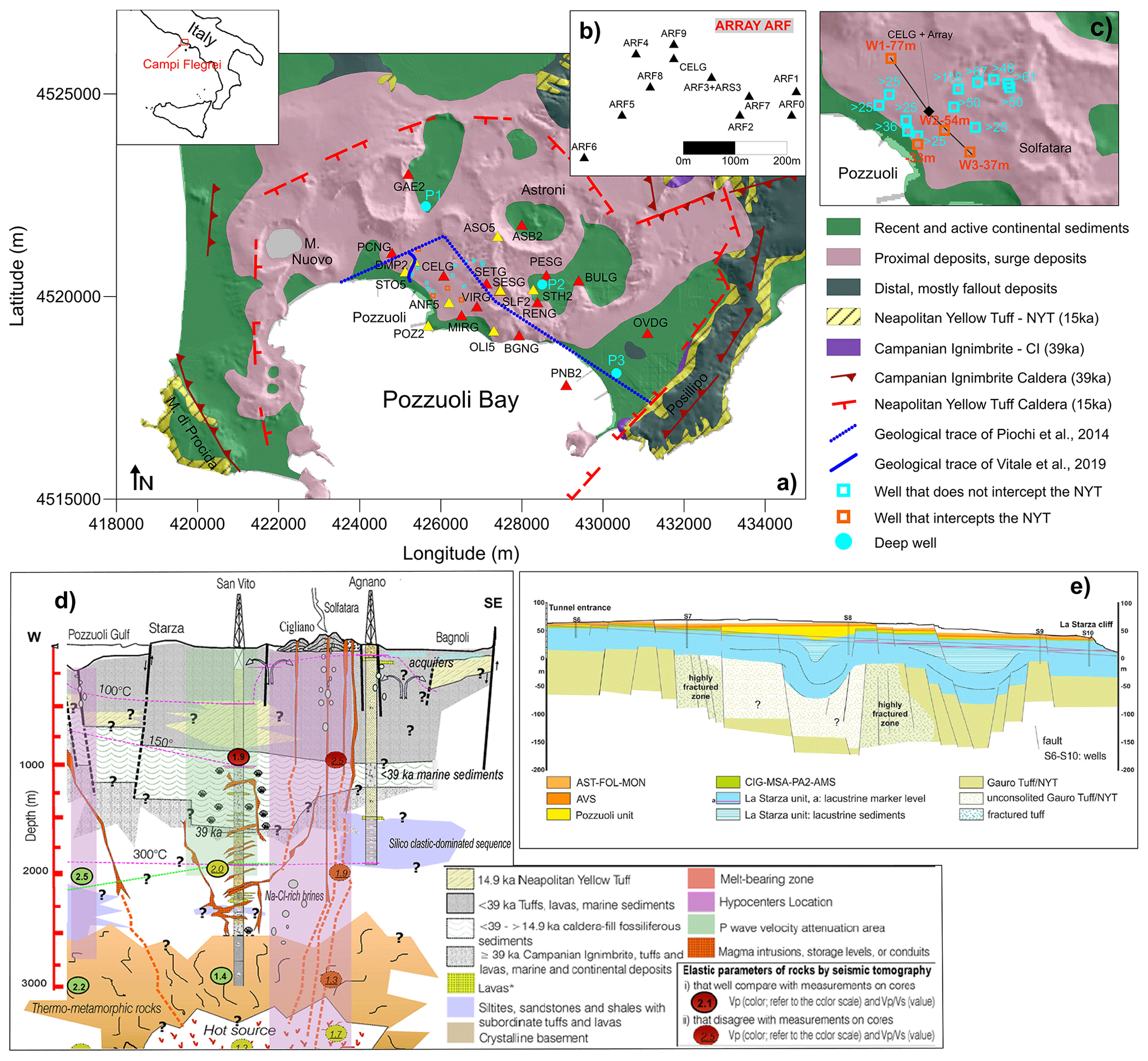
Figure 1 (a) Simplified geological map of Campi Flegrei area (modified after Orsi et al., 1996). The red and the yellow triangles are the stations used in this study of the Mobile Seismic Network (MSNt) and UNREST experiment (PSNt) installed in the Campi Flegrei area. (b) Configuration of the underground array “ARF”, installed together with the station CELG at 25 m depth, and the station ARS3, installed at surface, above ARF3. The cyan dots are the locations of the deep drilled boreholes: (1) S. Vito Well; (2) Agnano Well; (3) CFDDP well (De Natale et al., 2016).. The blue dotted line indicates the profile of the geological section/interpretation (d) of Piochi et al. (2014), reported in Fig. 10. The blue line is the trace of the geological cross section (e) of Vitale et al. (2019). (c) Zoom of the central area around the underground array, with some stratigraphic wells drilled after the 1980 bradyseismic event (Ducci and Rippa, 1988). The orange ones (W1, W2 and W3) intercept at the indicated depth (77, 54 and 37 m) the Gauro Yellow Tuff. The cyan ones, instead, do not intercept the Gauro Yellow Tuff, that is located at depth higher than those reached by the bottom of the wells (depths specified near the squares). The black line is the trace of the geological section reported in Fig. 9.

The outcropping rocks are composed by continental and marine sediments intercalated with pyroclastic deposits mainly emplaced by pyroclastic density currents in the proximal areas, and by pyroclastics fallout in the distal ones (Orsi et al., 2004, and references therein). These deposits are composed by loose pyroclastic material (ash, pumice, scoriae, lithics) or lithified tuffs and minor lavas. These sequences are intercalated, in the lowlands, with marine and coastal sediments (Di Vito et al., 1999). This complex structure built up by the overlapping of volcano structures and sediments make the Campi Flegrei an interesting site to study in terms of shallow (up to 200 m depth) and intermediate (up to 2000 m depth) velocity structures. The caldera structure has been object of several scientific studies aimed at the investigation of different and complementary parameters: identification of volcanic tremor of hydrothermal origin (De Lauro et al., 2013; La Rocca and Galluzzo, 2017), tomographic studies, using both active and passive data (Battaglia et al., 2008), noise based monitoring (Zaccarelli and Bianco, 2017), joint analysis of seismicity and ground deformation (De Lauro et al., 2018; Ricco et al., 2019; Petrosino et al., 2020), gravimetric (Capuano et al., 2013) and magnetic surveys (Florio et al., 1999) and deep magnetotelluric survey (Troiano et al., 2014). Recent studies of seismic attenuation (De Siena et al., 2010, 2017) reveal the existence of melted rocks at 4–5 km depth that are not shown by the seismic tomography. The presence of these volumes is in agreement with the evidence of petrological and geochemical data. Chiodini et al. (2016) explain the trend of the geochemical data suggesting the presence, beneath the Solfatara volcano, of a hydrothermal system at 2 km depth, which feeds two surface fumarolic areas. Indeed, the important role of the fluids in controlling the dynamics of the caldera has also been highlighted in several recent studies (e.g. Cusano et al., 2008; De Lauro et al., 2012, 2013; Petrosino et al., 2018). Given the complexity of the caldera highlighted by geophysical, geochemical and geological studies, an average 1D S wave velocity model would not be representative for the entire area of the Campi Flegrei. However, in this work the stations configuration allows to investigated the subsoil structure (down to 2000 m) of the central part of the Campi Flegrei area (Fig. 1), for which we expect the lowest variation in the structural settings. This goal was pursued by the application of array and spectral ratio techniques on seismic noise recordings, from the underground array ARF and from the broadband stations of the mobile seismic network and the UNREST experiment, which are considered as two large 2D seismic arrays. To avoid making mistakes when applying such specific methods, which require a 1D layered earth, we checked that the major seismic velocity and/or structural discontinuities are smaller than the minimum wave length resolution. As suggested by Nardone et al. (2020), despite the presence of lateral heterogeneities the 1D velocity profile can be considered as a good approximation of the velocity structure since it carries information about the average properties of the crust (Spica et al., 2015, and reference therein). An accurate velocity model for the first kilometres of the crust allows a better location of the volcanic processes (Bean et al., 2008) and can have significant implications for better understand the internal dynamics of the volcano, thus improving the interpretation of monitoring observations. This is particularly important in a high volcanic risk area such as Campi Flegrei.

2 Dataset and array resolutions

In this study we used three datasets: one recorded by the seismic array “ARF” (right inset in Fig. 1), one recorded by the Mobile Seismic Network (MSNt, red triangles in Fig. 1, La Rocca and Galluzzo, 2015) of INGV – Osservatorio Vesuviano and one by the seismic stations of the UNREST experiment (PSNt, yellow triangles in Fig. 1, Bianco et al., 2010). The monitoring network and the stations of the UNREST experiment are considered as two large arrays and their broad frequency bands, reaching frequency lower than 0.1 Hz (see Table 1), allow longer wavelength signals to be gathered and greater investigation depths compared to the array ARF.

Table 1 Geometry and technical characteristics of the three arrays.

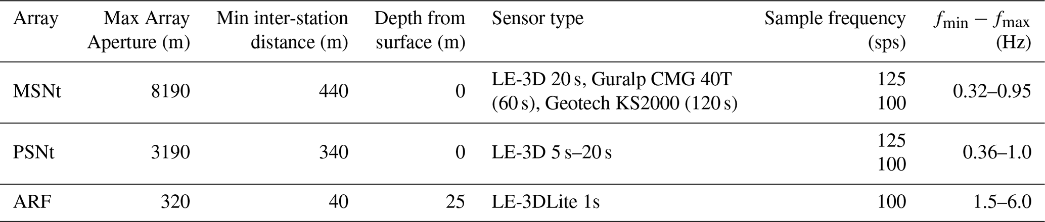
The minimum and maximum resolvable wavelength, respectively k_min∕2 and k_max, are directly related to the geometry of the arrays (inter-station distance and aperture), and they were estimated from the array transfer function (Di Giulio et al., 2006; Wathelet et al., 2008) (Fig. 2).

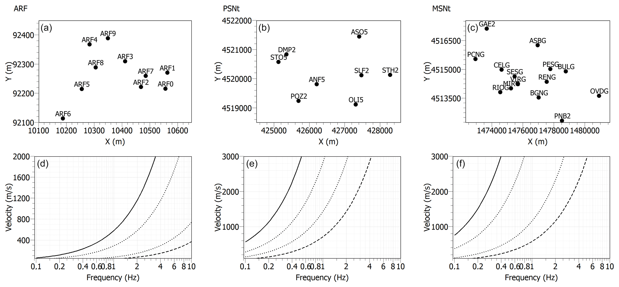
Figure 2 (a–c) 2D Arrays geometry; (d–f) resolution curves (k_min: thick dashed line; k_max: thick line; $k_{\max /\mathrm{2}}=k_{\mathrm{mix}/\mathrm{2}}$: dotted line).

The investigation depth depends on the maximum measured wavelength, and the resolution decreases with depth. In particular, the resolution at shallow depth depends on the high frequency content (small wavelengths) of the recorded data. The lower frequency limit (about 0.3 Hz for MSNt array) is the lowest frequency resolvable by the array and it is linked to the maximum distance between sensors (see Table 1). The seismic noise recordings cover at least 3 h, acquired in the following periods:

1. January 2011 (ARF plus ARS3 station)

2. October 2012 (PSNt)

3. August 2017 (ARF)

4. April 2018 (MSNt)

3 H∕V analysis

The array ARF installed underground is composed of six 3-component short period seismic stations connected to a 18-channel acquisition system, which acquired continuously at 100 sps (La Rocca and Galluzzo, 2012). The array was operating from 2010 to 2018. In the same area a surface free-field station “ARS3” (3-component short period) was installed for a few months during 2011. Since 2013 the number of vertical sensors was increased up to ten, but the 3-component stations were reduced to four (ARF1, ARF3, ARF4 and ARF6). We calculated the H∕V spectral ratio over 24 h of seismic noise samples acquired on 15 January 2011. Each 3-component recording was bandpass filtered in the 0.5–20 Hz frequency band and an STA/LTA algorithm was applied in order to reject transients and disturbances. Time-windows of 100 s with an overlap of 25 % were selected. The Fourier spectra of the NS and EW components were geometrically averaged to obtain the horizontal component Fourier spectrum. Thus, the spectral ratios between the horizontal and vertical components for each time-windows, smoothed by a Konno-Omachi function (Konno and Omachi, 1998), were calculated for all the stations (H∕V in Fig. 3 panels 1–6). The final H∕V curve (Fig. 3 panel 9) was obtained from the arithmetic mean of all the spectral ratios retrieved from the six underground stations (coloured H∕V in Fig. 3 panel 8). According to the criteria defined in the SESAME European Project Deliverable D23.12 (available from https://www.earth-prints.org/bitstream/2122/8423/1/Del-D23-HV_User_Guidelines.pdf, last access: 28 October 2020), we verified that number and length of the selected time-windows ensure the reliability of the H∕V curves. Moreover, we also checked that the obtained H∕V peak satisfies the amplitude and stability conditions indicated in the above-cited report, for an unambiguous and correct identification of the resonance frequency. The comparison of H∕V spectral ratio calculated in different periods of the year 2011 as well as in 2012 (for the available 3-component stations) shows no difference, indicating that the spectral ratios relative to January 2011 are stable in time.

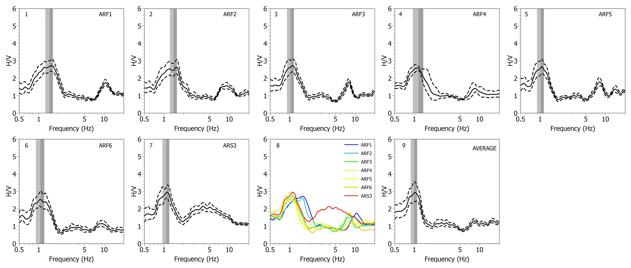
Figure 3 Panels from (1) to (6) are the H∕V spectral ratios of the six array underground stations (ARF*) and panel (7) is the H∕V spectral ratio of the surface station ARS3. The black continuous line is the mean of the H∕V spectral ratio. The dashed black lines are the standard deviations. The grey band identifies the f₀ frequency. In panel (8) the colors from blue to orange are the mean H∕V of the six underground stations and the red one is the mean of the surface station ARS3. In the panel 9 the array averaged H∕V is shown.

All the sites sampled by the six stations of the array show similar values of the fundamental frequency (1.0–1.4 Hz) and low average peak amplitude (2–3) (Fig. 3 panel 8). Interesting is to note the behaviour of the surface station, ARS3, whose H∕V curve shows a secondary broad peak in the 2–10 Hz frequency range (red curve in Fig. 3 panel 8). This is in agreement with the observation by La Rocca and Galluzzo (2012), that the underground H∕V spectral ratio is smaller than at surface particularly in the 2–5 Hz band, indicating that the noise is mainly composed by Rayleigh waves which quickly attenuates fastest with depth, and it is probably due to resonance caused by sediments located above the ARF array.

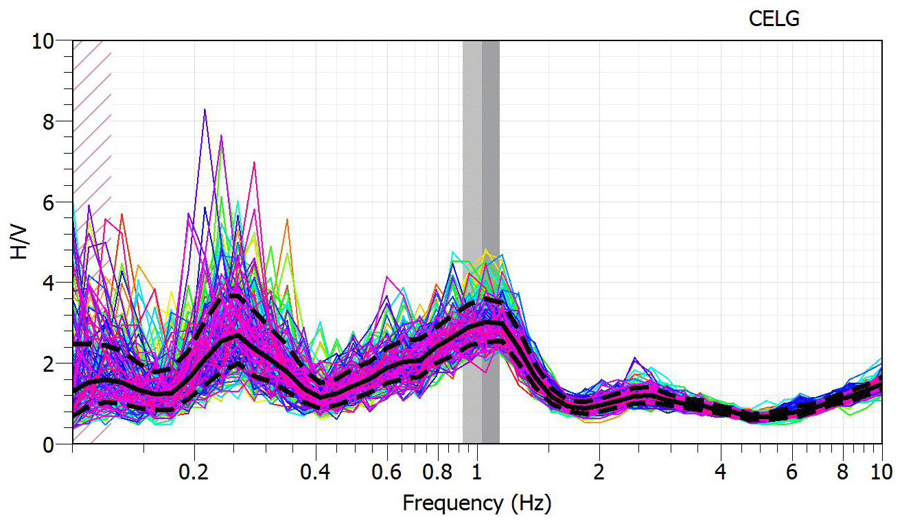
Figure 4 H∕V Spectral ratios of the broad band station CELG. The black continuous line is the mean of the H∕V spectral ratio obtained at each time-window (thin colored lines). The dashed black lines are the standard deviations. The grey band identifies the f₀ frequency.

Finally, we calculated the H∕V spectral ratio of the seismic noise recorded by the underground 3-component broadband station CELG, installed in the central area of the ARF array. Data recorded for each component were bandpass filtered in the 0.1–10 Hz frequency band, and the H∕V spectral ratios were calculated on 100 s moving time-windows with 25 % overlap. The final H∕V curve (Fig. 4) was obtained from the arithmetic mean of all the spectral ratios retrieved from the analysed time-windows.

4 Dispersion curve estimates

We estimated the dispersion curves of Rayleigh waves propagating through the arrays by applying the f–k technique (Lacoss et al., 1969). In order to compare days with low anthropogenic activity to those characterized by higher level of human-generated seismic noise, we used data recorded on Sundays and Mondays of August 2017 by the ARF Array. For each day, we bandpass filtered the 24 h long recordings (vertical component) in the 0.5–8 Hz, choosing values of center frequency, f_c, with step of 0.1 Hz and bandwidth defined as 0.9f_c–1.1f_c. The time-window length was selected equal to 50 times the central period of each analyzed band, with an overlap between successive windows equal to 30 %. For each frequency band, the f–k spectrum was computed over a grid with size equal to k_max and step less than k_min∕4. The maximum of the f–k spectrum corresponds to the best slowness value: the values associated to all the selected time-windows at a fixed frequency were used to calculate the slowness mean value and its associated statistical error (Ohrnberger et al., 2004). The phase velocity dispersion curve of the fundamental mode of Rayleigh waves was obtained by plotting the inverse of slowness as a function of frequency and selecting the part of the curve bounded by the resolution limits defined through k_min and k_max. No difference between dispersion patterns retrieved on Sundays and Mondays was observed, thus indicating that different levels of anthropogenic noise do not affect the shape of the dispersion curves. The final dispersion shows phase velocity ranging from about 1100 m s⁻¹ at frequency of 1.4 Hz to about 200 m s⁻¹ for frequencies higher than 4 Hz and up to 6 Hz (Fig. 5). To further validate the dispersion results obtained with the f–k technique, we applied the SPatial AutoCorrelation (SPAC) method (Aki, 1957, 1965) in the version modified by Bettig et al. (2001), MSPAC, to the same data-set. Since ARF array was modified in 2013 including 10 vertical component stations, all the possible combinations (without redundancies) of station pairs are 45, were arranged in three distance ranges (rings). For each ring we estimated the average autocorrelation coefficient, using the signals recorded at the vertical components, filtered in the band 0.5–8 Hz and divided in time-windows with a length of 50 times the central period of each analysed frequency band, with an overlap of 30 %. For each day we obtained three autocorrelation coefficients, one for each ring, as functions of frequency, containing 40 samples linearly spaced over the band 0.5–8 Hz. The procedure of fitting the 0-order Bessel function produces a semblance function in the slowness-frequency plane. The Rayleigh wave fundamental mode dispersion curve was obtained by picking the maxima of this function, in the range of the k_max and k_min curves, to avoid the picking of aliasing false maxima. The final dispersion curve was calculated by averaging all the picked curves (continuous white line in Fig. 5).

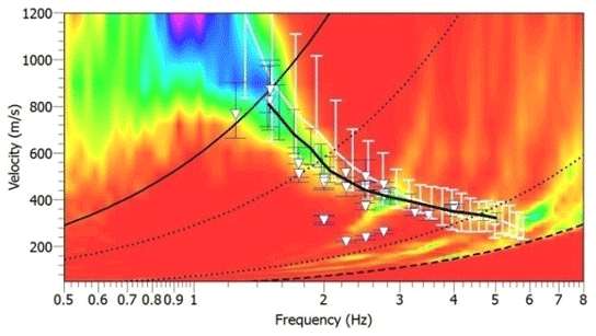
Figure 5 Dispersion curve of the array ARF. The black curve is the picked dispersion curve with relative error bars. The white curve is the dispersion curve obtained applying the MSPAC method to the same dataset. The white triangles are the phase velocities derived from the analysis of the coherent transient signals. The resolution curves are: k_min: thick dashed line; k_max: thick line; $k_{\min /\mathrm{2}}{k}_{\max /\mathrm{2}}$: dotted line.

Inside the error bars, the average MSPAC and f–k curves are comparable. Further constraints on the dispersion curves are obtained from the estimate of the phase velocity of coherent transient signals recorded by the array (white triangle in Fig. 5). Array analysis of continuous recordings revealed the occasional presence of coherent signals that propagate through the array as surface waves. They are attributed to artificial sources widespread in the area, and are characterized by frequency in the 1.2–4 Hz range, and scattered backazimuth. An example of such coherent signals is shown in Fig. 6 of La Rocca and Galluzzo (2015). Finally, we applied the f–k method to the vertical component of the seismic noise continuously recorded during October 2012 and April 2018 by the PSNt and MSNt arrays, respectively. We bandpass filtered the 24 h long recordings in the 0.1–2 Hz, choosing values of center frequency, f_c, with step of 0.1 Hz and bandwidth defined as 0.9f_c–1.1f_c. The time-window length was selected equal to 500 times the central period of each analyzed band, with an overlap between successive windows equal to 30 %. The phase velocity dispersion curves of the fundamental mode of Rayleigh waves were obtained by plotting the inverse of slowness as a function of frequency and selecting the part of the curve bounded by the resolution limits defined through k_min and k_max (Fig. 6).

Figure 6 Picked dispersion curves (black continuous line) with relative error bars obtained for MSNt and PNSt. The dotted line is $k_{\min /\mathrm{2}}=k_{\max /\mathrm{2}}$, the thick dashed line is k_min and the thick is line k_max.

Thanks to the larger dimension of the arrays and to the broad frequency band of the seismometers (see Table 1) the final dispersions reached phase velocity values of about 2300 m s⁻¹ at frequency of about 0.3 Hz (MSNt) and about 1900 m s⁻¹ at frequency of about 0.35 Hz (PSNt). The lowest velocity value is around 800 m s⁻¹ at about 1 Hz for both the arrays.

As a final step all picked dispersion curves obtained from the f–k analysis, from MSPAC, as well as the single phase velocity values derived from the analysis of coherent transient signals were averaged, smoothed and resampled in a final dispersion curve (Fig. 7).

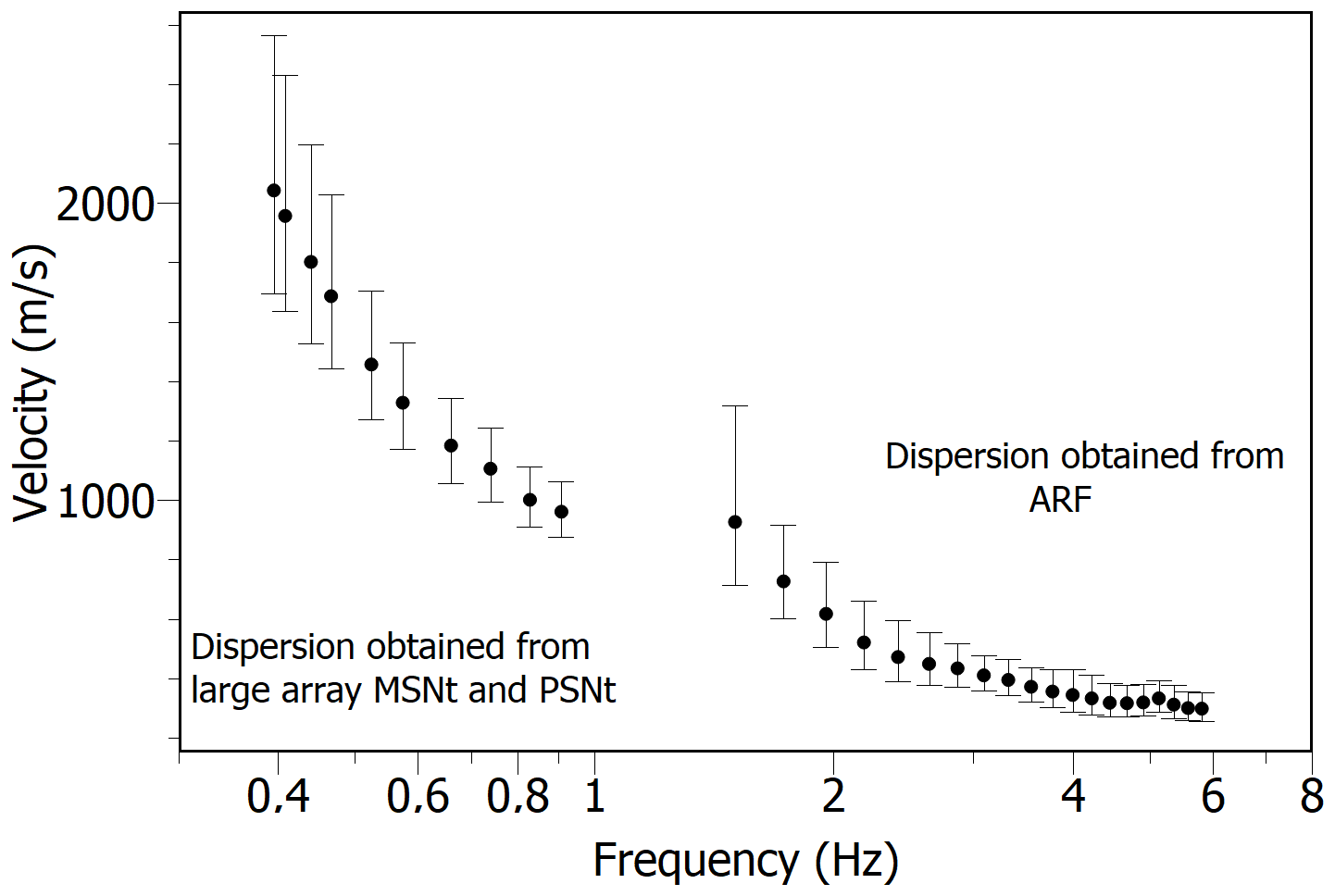
Figure 7 Observed phase velocity obtained averaging the dispersion values estimated from the f–k analysis applied to PSNt and MSNt arrays (Fig. 6), and the f–k and MSPAC analysis plus the single phase velocity values derived from the analysis of coherent transient signals, for the array ARF (Fig. 5).

5 Inversion procedure

We applied the neighbourhood algorithm (Sambridge, 1999) implemented by Wathelet et al. (2004, 2005, 2008), which infers the best velocity model (selected considering the minimum of the misfit function) through a stochastic search in a multi-parameter space. Each point of this space is defined by S and P wave velocities, top depths, densities and Poisson's ratios of the soil layers, and hence, each point of the space represents a theoretical velocity model. The best parameters (or equivalently, the best model) are derived by an inversion procedure, fitting the experimental dispersion curve with a theoretical one, as the parameters vary over the parameter space. To better constrain the inversion procedure of the obtained averaged dispersion curve in the 0.3–6 Hz frequency band, the H∕V curve and the resonance frequency (whose value depends on the layer thickness and shear-wave velocity; Kramer, 1996) of the station CELG have been used. In a preliminary study, Nardone et al. (2017), using ambient noise records of ARF array jointly inverted with H∕V ratio of coda waves of earthquakes recorded at CELG station, obtained a preliminary model composed of three main layers over a half-space with a shear-wave velocity increasing with depth. Starting from the results found by Nardone et al. (2017), we performed the inversion process, modifying the constrain on the space of the parameters and considering the evolution of the misfit as a function of V_S and thicknesses. During the inversion procedure, the possibility of adding another layer has been explored by modifying the constraint on the space of the parameters and considering the evolution of the misfit as a function of V_S and thicknesses. We have chosen to modify only these two parameters as they have the greatest influence on the dispersion curve (Wathelet et al., 2005).

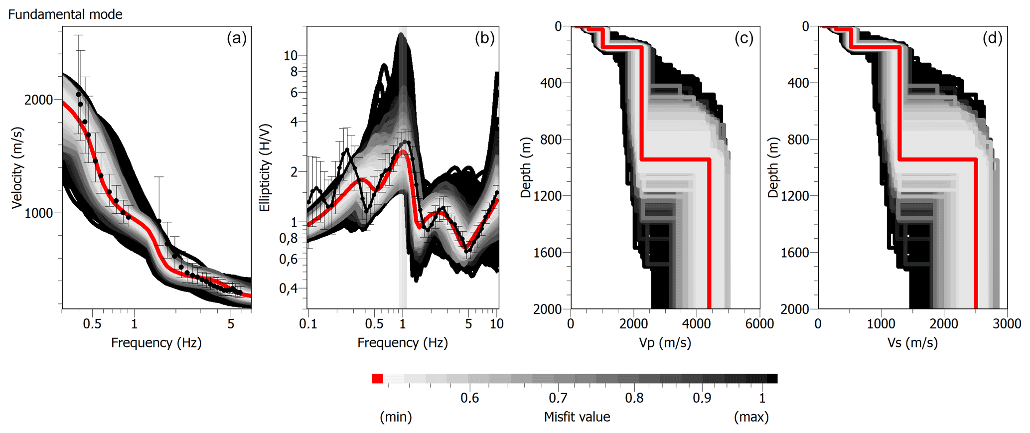
Figure 8 Results of the joint inversion of averaged dispersion curve and H∕V data. (a) Observed phase velocities (black dots) and relative error bars, phase velocities for the minimum cost model (red line), and phase velocities for the space of stable generated models (gray band). (b) Mean H∕V (black dots) and relative error bars, ellipticity function for the fundamental mode of Rayleigh waves for the minimum cost model (red line), and ellipticity functions for the space of stable generated models (grey band). The grey vertical band identify the mean frequency peak f₀. (c) and (d) minimum misfit P and S wave velocity models (red line) and space of stable generated models (grey band).

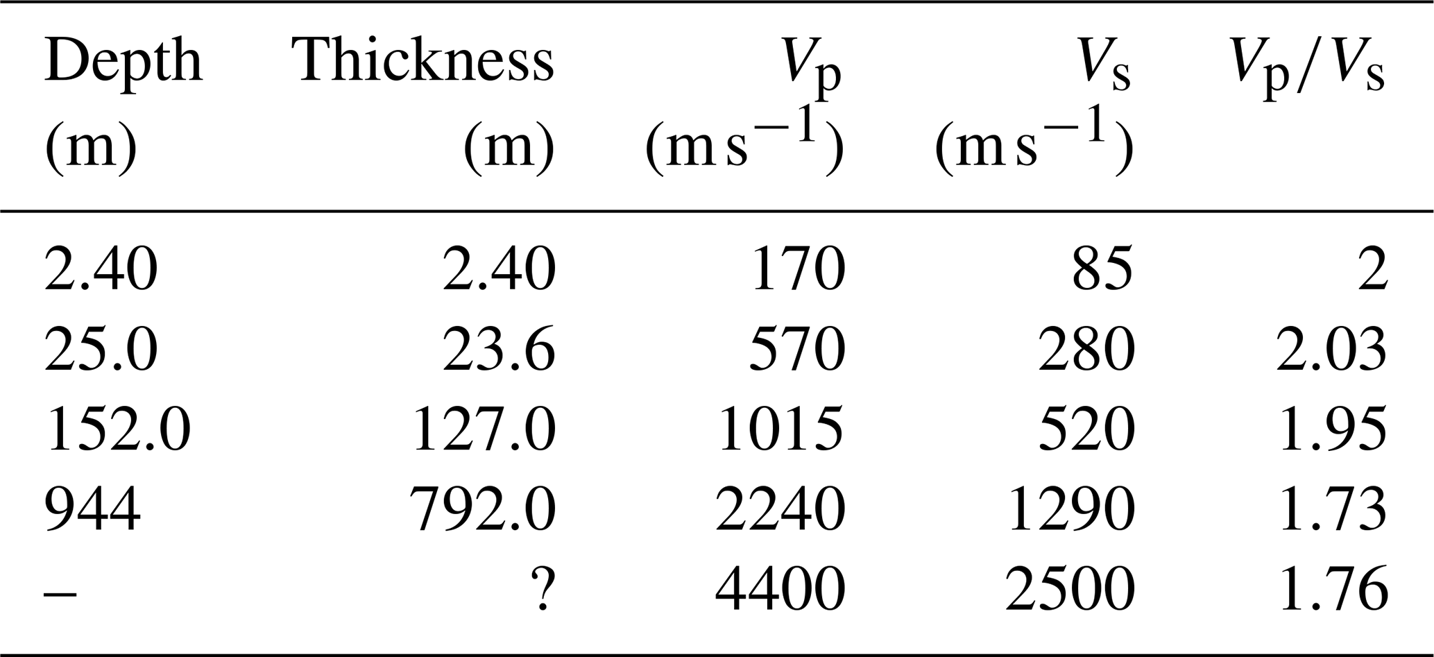
The models resulting after 13 inversion processes show a good fit (minimum misfit = 0.515) between experimental and theoretical curves by using a parameterization of four main layers over a half-space with a shear-wave velocity increasing with depth (Fig. 8 and Table 2). The final seismic velocity model has a higher resolution for the shallower layers (first 100–200 m) compared with the deeper ones.

6 Geological interpretation

In order to interpret the velocity model obtained from the joint inversion of dispersion curve and H∕V spectral ratio in terms of the geological information, we differentiate between shallow (200 m) and deep (up to 2 km depth) structure using data from both the stratigraphy of shallow wells (up to about 90 m depth; Ducci and Rippa, 1988) and three deep boreholes for geothermal exploration. The lithological reconstructions of the central part of the caldera, reported in Piochi et al. (2014) from a re-evaluation of the original reports on the AGIP boreholes and from lithological information from the SAFEN Agnano drill hole, were the starting point. We also used the stratigraphic section reported in Vitale et al. (2019) to better constrain the shallower layers.

Table 2 The velocity profile with the lower misfit value (0.515).

Shallow structure. We identified the depth of the Gauro Yellow Tuff top using the wells drilled around the array site (Fig. 1).

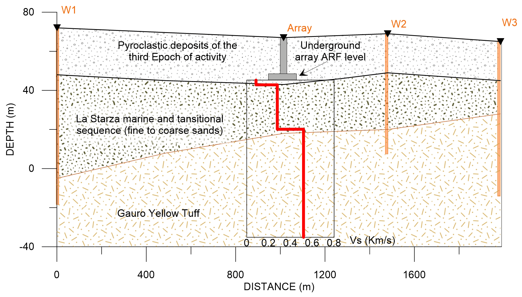
Figure 9 Geological section along the black line reported in the inset in Fig. 1, obtained from stratigraphic information coming from wells (orange squares in the zoom of Fig. 1) and from shear wave velocity model achieved from the joint inversion.

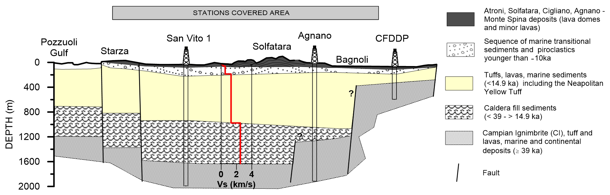
Figure 10 Large scale geological interpretation modified after Piochi et al. (2014), along the blue dotted line reported in Fig. 1. The contact between the principal lithological sequences are inferred from the stratigraphic information of the deep drills. The best model obtained from the joint inversion (Fig. 8 and Table 2) is reported with the red line.

The deepening of the tuff top in the NW direction is also confirmed by the depth obtained from the velocity model. The first seismic layer (Table 2) is interpreted as composed mainly of loose pyroclastic deposits of the third epoch of activity (Di Vito et al., 1999; Roberto et al., 2015). The second seismic layer has been associated to the marine and transitional sequences (La Starza terrace), that include fine to coarse-grained sands with intercalations of lenses and layers of pumices, scoriae, and pebbles (Fig. 9). At the base there is the massive Gauro Yellow Tuff (<15 ka, Fig. 9). The velocities obtained for these shallower layers are comparable and coherent with those found for both pyroclastic deposits and lithified facies of the Neapolitan tuffs (Petrosino et al., 2012; Maresca et al. 2013; Costanzo and Nunziata, 2019). Since we do not have a direct measure of the depth of the tuff (all the cyan wells, indicated with square symbols, in Fig. 1 do not intercept it), we cannot extend certainly this shallow reconstruction for the whole investigated area, but only for a small part. We are sure about the uniformity of the subsoil below the array ARF, because we checked the stability of the H∕V curve along the array (as suggested by Foti et al., 2017). A 1D hypothesis for the area sampled by the array ARF is justified because the shapes of H∕V curves are the same (Fig. 3 panel 8), indicating a homogeneity of the sampled subsoil.

Deep structure. At larger scale, three deep boreholes drilled for geothermal exploration, has been used to constrain the geological interpretation (Fig. 10) of the deeper velocity structure. Further information was obtained using the geological sections available for the area (Piochi et al., 2014). The velocity model obtained as a result of this study matches the two geological interfaces represented in the geological section of Fig. 10. The shallow one (around 150 m depth, corresponding in the H∕V curve to the peak at 1 Hz) is between the subaerial pyroclastic deposits, the marine-transitional sequence of la Starza Unit and the Gauro Yellow Tuff, overlaying tuff (Neapolitan Yellow Tuff), lavas and marine sediments younger than 39 ka. The latter is separated from the caldera fill sediments (<39 ka to >14.9 ka) by a second surface located at 1000 m depth. This last surface is probably responsible of the peak around 0.25 Hz of the CELG station H∕V curve (Fig. 4).

The large scale geological information, integrated with the velocity model derived from the joint inversion (cf. Sect. 5), allowed us to reconstruct the stratigraphic geometry of the investigated area, up to a maximum depth of 1600 m. Our expected maximum depth of investigation (P_max) depends on the maximum experimental wavelength ($\mathit{\lambda }max=\sim \mathrm{5000}$ m at 0.4 Hz) like $\sim \mathit{\lambda }max/\mathrm{3}$ to $\mathit{\lambda }max/\mathrm{2}$. As suggested by Foti et al. (2017) the maximum depth can be less than P_max in stratigraphic conditions involving large impedance contrast at depth, and this could be the reason why we have not been able to identify the top of the Campania Ignimbrite (1600 m depth).

7 Conclusion

In this work we provide a more detailed velocity model for the central part of the Campi Flegrei caldera using surface wave dispersion and spectral ratio of seismic noise. Performing a joint inversion, involving both dispersion curves, ellipticity curve and value of fundamental frequency f₀, we have reduced the uncertainty on the best-fit model due to the non-uniqueness of the solution. Furthermore the obtained velocity model has been interpreted using geological constraints (such as deep boreholes) to confirm the 1D hypothesis at large scale (Fig. 10), that allow us to assume this model as representative for the whole investigated area. The 1D assumption is not valid at shallower scale (Fig. 9), within the 200 m depth. In fact in this case the stratigraphic information highlights the variability of the top of the Gauro Tuff, ruling out the assumption of a 1D stratification (Fig. 9). Indeed, Vitale et al. (2019) have reconstructed the tectonostratigraphic architecture of the Pozzuoli northern area using field geological investigations, integrated with information from well logs and ERT surveys, getting a complex geometry characterized by faulted tuff blocks, particularly in the first 150 m depth (Fig. 1e). Furthermore, the complex geometry of the superficial layers is also confirmed by the velocity model obtained by Petrosino et al. (2012) for the Solfatara area, which is about 1500 m away.

The velocity model obtained in this study is reliable and realistic if compared with other published results for the Campi Flegrei volcanic area. Costanzo et al. (2017), using noise cross-correlation analysis and non-linear inversion of fundamental-mode Rayleigh waves, obtained V_S profiles of the first 2 km depth. The values retrieved by the authors for the caldera central part are comparable to those found in this study, particularly for the fourth seismic layer associated to the tuff (Neapolitan Yellow Tuff), lavas and marine sediments younger than 39 ka. A recent study (Calò and Tramelli, 2018) using the data of the last bradyseismic event have recognized shallow high V_P∕V_S ratio (>1.85) volumes in the center of Campi Flegrei caldera, interpreting as due to the presence of shallow reservoirs mainly water saturated. The V_p∕V_s ratio of the model obtained in our study (Table 2), ranging between 1.76 (for the half space) and 2 (for the shallowest layers), is consistent with that obtained by Calò and Tramelli (2017), but we are not able to distinguishing the presence of water. More observation on dispersion curves are needed to define the possible variation on Rayleigh wave phase velocity caused by the hydrogeological oscillation of the shallow reservoir.

The results of the present study provide a quantitative estimate of the parameters that control the propagation of waves in a complex volcanic area, in which detailed knowledge of the elastic properties of the subsoil represents one of the fundamental objectives to understand its dynamics. In particular, improved imaging of volcanoes leads to a better interpretation of volcanic processes, a better description of magmatic systems dynamics, and thus an improved assessment of the associated hazards.