GIS applications in volcano monitoring: the study of seismic swarms at the Campi Flegrei volcanic complex, Italy

Campi Flegrei caldera (Southern Italy) is one of the most hazardous volcanic complexes in the world since it is located inside the densely inhabited urban district of Naples-Pozzuoli. In the past, the caldera has produced devastating to moderate eruptions and periodically undergoes from strong to minor uplift episodes, named “bradyseism”, almost always accompanied by seismic swarms. Starting from 2005 Campi Flegrei has undergone an unrest crisis, characterized by ground uplift, localized gas emissions and seismicity, often occurring in seismic swarms. As a consequence, the monitoring activities have been progressively increasing, producing a huge amount of data, difficult to manage and match. GIS (Geographical Information System) represents a potent tool to manage great quantity of data, coming from different disciplines. In this study, we show two GIS technology applications to the seismic catalogue of Campi Flegrei. In the first one, a high-quality dataset is extracted from the GeoDatabase addressed to seismological studies that require high precision earthquake locations. In the second application, GIS are used to extract, visualize and analyse the typical seismic swarms of Campi Flegrei. Moreover, density and seismic moment distribution maps were generated for these swarms. In the last application, the GIS allow to highlight a clear variation in the temporal trend of the seismic swarms at Campi Flegrei.

1 Introduction

Campi Flegrei (CF) caldera is one of the most hazardous volcanic area in the world (Orsi et al., 2004), belonging to the densely urbanized settlement of Naples and Pozzuoli cities (Southern Italy, Fig. 1). The caldera has been modelled over the time by several devastating or moderate eruptions. The most destructive ones occurred about 40 ka, the Campanian Ignimbrite, and about 15 ka, the Neapolitan Yellow Tuff, while the most recent, Monte Nuovo eruption, took place in 1538 (Di Vito et al., 2016). Del Gaudio et al. (2010), through an historical reconstruction of the ground deformation at CF over the last century, found that several cycles of uplift/subsidence, termed “bradyseisms”, interested the caldera accompanied by seismic activity. In recent times, the most severe bradyseismic crisis occurred in 1982–1984 (Del Gaudio et al., 2010), starting with a rapid ground uplift, whose peak was reached in 1983, shortly followed by an earthquake of M= 4.0, the stronger seismic event recorded in CF until nowadays. At the end of 1984 the uplift reached its maximum (1.79 m) and then a subsidence stage started, and the seismicity declined. Sometimes, the overall subsidence has been interrupted by miniuplift, or “unrest” episodes (Del Gaudio et al., 2010), always along with seismicity.

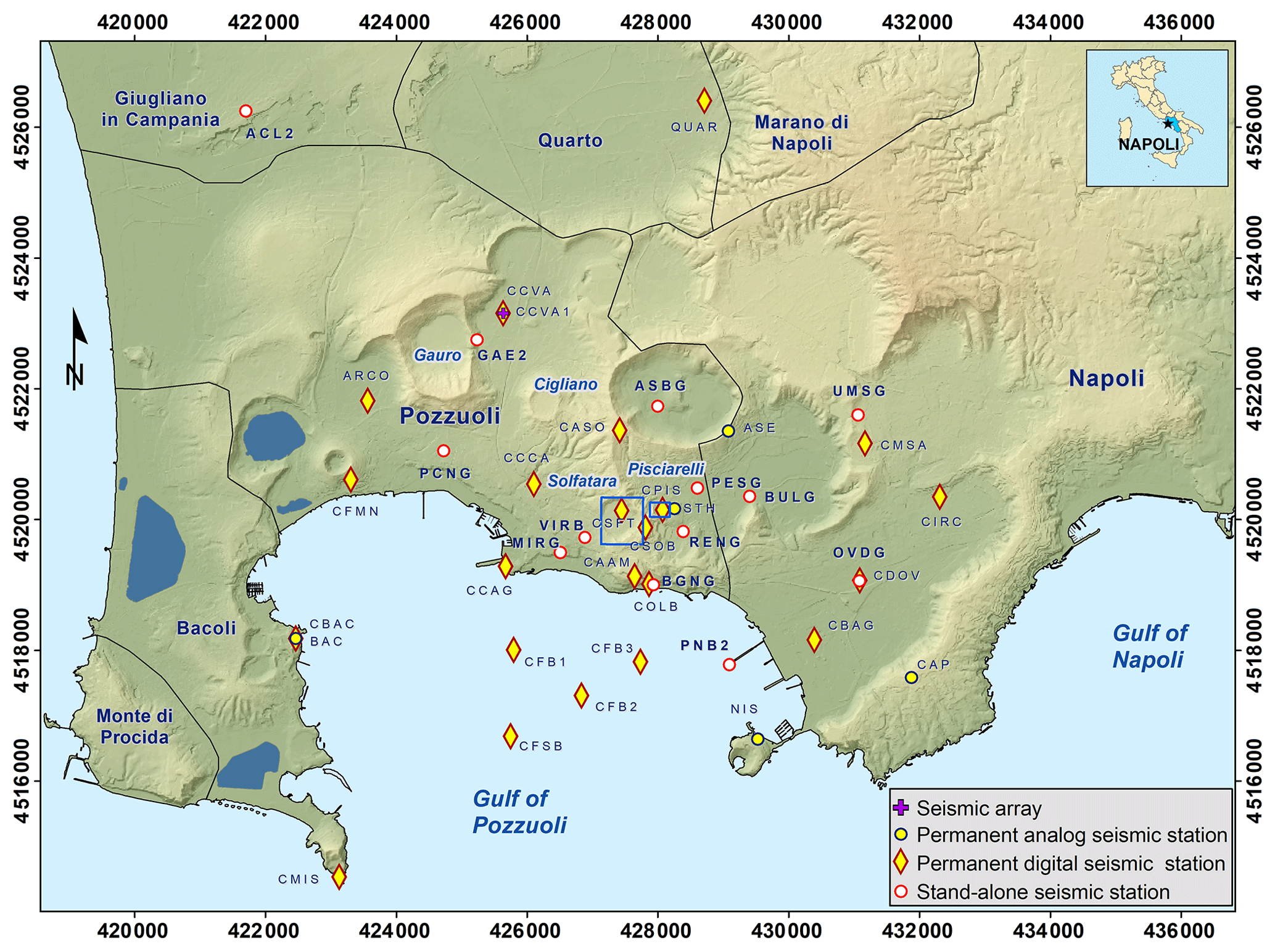
Figure 1 Study Area. Reference system UTM WGS84. The blue squares highlight the Solfatara crater and Pisciarelli area. The seismic stations are indicated according to the legend on the bottom right. In the upper right corner the position of study area inside the Italian territory is shown. Digital Terrain Model (DTM) of Campi Flegrei (Vilardo et al., 2013).

A new ground uplift phase started in 2005 and it is still ongoing, with a total vertical displacement of 63 cm recorded at the end of 2019 (Bevilacqua et al., 2020). This unrest is monitored by the most modern surveillance networks of Istituto Nazionale di Geofisica e Vulcanologia – Osservatorio Vesuviano (INGV-OV) of Naples (http://www.ov.ingv.it, last access: 20 December 2020). Besides the seismic activity, the current bradyseism presents also an increasing degassing activity and variations in the composition of the fluid emissions (Tamburello et al., 2019, and references therein), mainly in the hydrothermal areas of Solfatara and Pisciarelli (Fig. 1). Chiodini et al. (2016) proposed a physical model that links all the surface manifestations to the dynamics of the magmatic-hydrothermal system. Those authors hypothesize the existence of a gas accumulation volume at about 4 km of depth, related to magmatic fluid pressure into the plastic zone or to magmatic batches. The volume releases hot gases toward the hydrothermal reservoir, located at about 2 km of depth, where the upwelling magmatic fluids mix to cold meteoric water and vaporize.

In 2012 an increase of the uplift rate, together with anomalous seismicity and strong degassing, was recognized. It was interpreted by different authors as caused by a magmatic intrusion at shallow depth (D'Auria et al., 2015; Chiodini et al., 2017). These circumstances induced the Italian Civil Protection Department (CPD) to move the volcanic alert level from “background” (“Green” Level) to “attention” (“Yellow” Level).

Geographical Information Systems (GIS) applications are fundamental to represent, inquire, select, match and analyse any kind of geographical information, being an essential tool for decision support.

With respect to other software packages, such as ZMAP (Wiemer, 2001) and OBSPY (Megies et al., 2011), which were developed to analyse seismic data (both catalogs and waveforms), GIS were conceived to organize and integrate huge quantities of multidisciplinary data and to easily create thematic and integrated maps. Therefore, ZMAP and OBSPY have the limitation to deal only with seismic data and the advantage to contain large libraries of functions to analyse the data. On the other side, GIS are developed to integrate and spatially represent a wide variety of data, as well as to perform simple analyses, such as statistics. In summary ZMAP/OBSPY and GIS can be considered complementary. Indeed, many users still use GIS/ArcGIS tools to graphically represent the results obtained with ZMAP or OBSPY, although ad hoc packages were developed for these software.

In the last two decades, several researches produced a considerable number of studies based on GIS applications for CF, mainly devoted to volcanological field and volcanic hazards, often associated to the prediction of the most probable eruption following a renewal of volcanism over several time scales. Orsi et al. (2004) used the pyroclastic dispersion and load maps, generated in GIS environments, to identify areas susceptible to the opening of a new vent, zones that could be affected by variable load of fallout deposits, and areas over which pyroclastic currents could flow. A preliminary version of their study was adopted as the scientific basis for the development of an Emergency Plan by the CPD. By using GIS software, Alberico et al. (2002), evaluated the interaction between the energy of the expected eruptions and the CF caldera topography, obtaining risk maps by superposing hazard maps on urbanization map. Selva et al. (2012) constructed volcanic hazard maps in GIS environments, on the base of Bayesian inference scheme, merging prior information and past data. Bevilacqua et al. (2015) largely used GIS applications to produce probability maps of vent opening inside CF caldera on long-term scale or as rate basis. Since these maps permit to take into account for pyroclastic density currents and ash fallout, they represent a crucial starting point for the realization of probabilistic hazard maps. GIS products were also used by Neri et al. (2015), which produced hazard maps of probabilistic pyroclastic density currents invasion for the CF area, using a Monte Carlo simulation. The probability map of vent opening at CF was used as input data, together with the limits of the pyroclastic deposits of the last 15 ka, to simulate the possible area affected by the dispersion of the pyroclastic currents of a future eruption. Bellucci Sessa et al. (2008) have created a volcanological database containing all the information about the CF past eruptions available up to the date of the study. Data sources were heterogeneous: altimetric and geographic data (Regional Technical Map and DTM), geological and structural maps and bibliography, data from aircraft photographs, data from geological and structural surveys and data from laboratory analyses. These authors have homogenized and stored the data in a single database in a GIS environment, making the information easy to update and easy to use.

GIS applications were also developed and used in seismotectonic field. Pignone et al. (2007) imported the seismicity data recorded by INGV from 1981 to 2002 in GIS environment (CSI 1.0 1981–2002). The event density and energy release maps were generated easily and quickly. Those maps also represent a fundamental basis to support the mitigation of seismic hazard in Italy. For the assessment of seismic risk, Al-Dogom et al. (2018) used the geostatistical analysis tools of GIS to evaluate and analyse the spatial distribution of seismic events throughout the Arab plate. In particular, the directional distribution of earthquake magnitudes, the directional trend of earthquakes and the ground peak acceleration (PGA) were generated. These data were combined with fault line distance, slope, soil type and geology to identify seismic hazard zones. Kassaras et al. (2020) presented new Seismotectonic Atlas of Greece, harmonizing and integrating the most recent seismological, geological, tectonic, geophysical and geodetic data in an interactive, online GIS environment.

In this work, we show two applications of GIS technology to CF seismological data. In addition to the creation of a new GeoDatabase, containing seismic data from 2005 to 2019, the potential of GIS in the selection of earthquakes with high location quality is shown. Then, we demonstrate the GIS capability in performing: semi-automatic selections of the seismic swarms that have occurred at CF; reports that allow to quickly highlight the evolution of seismicity during the study period; maps of the epicentral density and the distribution of the seismic moment release of swarms.

2 Data and methods

2.1 Seismicity of Campi Flegrei

The CF seismicity is mostly composed of Volcano Tectonic (VT) earthquakes, with a high frequency spectral content (mainly > 6 Hz, up to 15 Hz) (Saccorotti et al., 2001; Iannaccone et al., 2001) and a prevailing brittle shear failure source mechanism (La Rocca and Galluzzo, 2019), probably caused by the pressurization of the hydrothermal system and the upwards fluid flow. Most seismic events have been located in the central part of the caldera, beneath the Solfatara-Pozzuoli area, where ground uplift shows the highest values, with depths up to 4 km b.s.l. (D'Auria et al., 2015; Petrosino et al., 2018).

In general, CF uplift episodes have been accompanied by VT seismicity, often occurring in swarms, which usually concentrates in a few hours or minutes, and less frequently by isolated earthquakes (Petrosino et al., 2018). By analysing the seismicity between 2000 and 2016, Chiodini et al. (2017) found that CF seismicity includes events with low inter-arrival time (< 15 min) corresponding to swarms, and high inter-arrival times (> 3 d) that are isolated earthquakes.

In recent times, the most severe seismic crisis occurred during the 1982–1984 bradyseism, with more than 16 000 VT events (maximum duration magnitude M_d= 4.0) mostly located beneath Pozzuoli town (Aster and Meyer, 1988). From 1989, the vertical movement alternates periods of increased uplift rate with intervals of subsidence or stationary conditions. These uplift phases have been associated with earthquakes, while the overall subsidence occurs aseismically (D'Auria et al., 2011, and references therein). Among the uplift episodes, the March–August 2000 crisis (maximum uplift of about 4 cm) presented Long Period events (LP, mainly frequency < 6 Hz), observed inside the CF caldera for the first time (Saccorotti et al., 2001; Bianco et al., 2004). After August 2000, the subsidence started again.

Regarding seismicity, during the current unrest phase (started in 2005) two main episodes should be mentioned. The first concerns the period January 2006–October 2007, during which a swarm of about 150 VT (Saccorotti et al., 2007) and 870 LP earthquakes (Cusano et al., 2008; Capuano et al., 2016) occurred. The VTs were mostly located at a depth of 2 km beneath Solfatara volcano, and the LP inside the crater at very shallow depth (Cusano et al., 2008; D'Auria et al., 2011). The second remarkable episode regards a strong accelerating rate observed in the period April 2012–January 2013. It was accompanied by a seismic swarm of about 200 VTs in 1.5 h on 7 September 2012, located in an area unusually affected by seismicity. Several authors (D'Auria et al., 2015; Di Luccio et al., 2015) associated this swarm with the reactivation of pre-existing faults by a magmatic intrusion beneath the CF caldera.

Our dataset consists of the VT earthquakes occurred inside CF caldera from 2005 to 2019 (Fig. 2, see Sect. 2.2), and acquired by the seismic network (Fig. 1) managed by INGV–OV. Since 2000 the network has undergone several technological improvements in response to the surveillance requirement derived from the ongoing unrest phase. Until 2014, the seismic network consisted of 17 permanent stations and 13 temporary stations, while at present the network is composed of 25 permanent and 13 temporary stations (http://www.ov.ingv.it/ov/it/bollettini.html, last access: 20 December 2020). Chiodini et al. (2017) noted that the development of the seismic network improved the quality of the hypocenter locations, but did not significantly affect the detection capability, because the station distribution was already effective since 2000. The permanent stations consist of both analog and digital instruments (Chiodini et al., 2017). The analog devices are equipped with short-period 1 Hz seismometers, while the digital stations are coupled with three-component broadband seismometers. The signals are telemetered in real-time to the Monitoring Centre of the INGV-OV in Naples, at a sampling rate of 100 Hz. The temporary stations (La Rocca and Galluzzo, 2015) consist of stand-alone dataloggers equipped with three-component short-period or broadband sensors. The data are locally acquired at 125 or 100 Hz sampling rate. Further details are available at the URL http://www.ov.ingv.it (last access: 20 December 2020).

The seismic signals are routinely picked by the analysts of INGV-OV Seismic Laboratory (http://sismolab.ov.ingv.it/sismo/, last access: 20 December 2020) and located by using HYPO71 (Lee and Lahr, 1972), that operates over a 1D velocity model covering the entire CF caldera. The Laboratory also estimates the duration magnitude M_d (Vilardo et al., 1991), calculated at the analog, shortperiod station STH. Chiodini et al. (2017) fixed the magnitude completeness equals to −1.0, which can be considered almost unchanged in recent years.

2.2 The new GeoDatabase in GIS environment

With the aim of predisposing a technological tool to support the management of the seismic events recorded inside CF caldera, we have converted the existing VT earthquake catalogue of INGV-OV (http://www.ov.ingv.it/ov/it/banche-dati.html, last access: 20 December 2020) from 1 January 2005 to 31 December 2019 in a GeoDatabase in ArcGIS© (ESRI) environment (rel. 10.6).

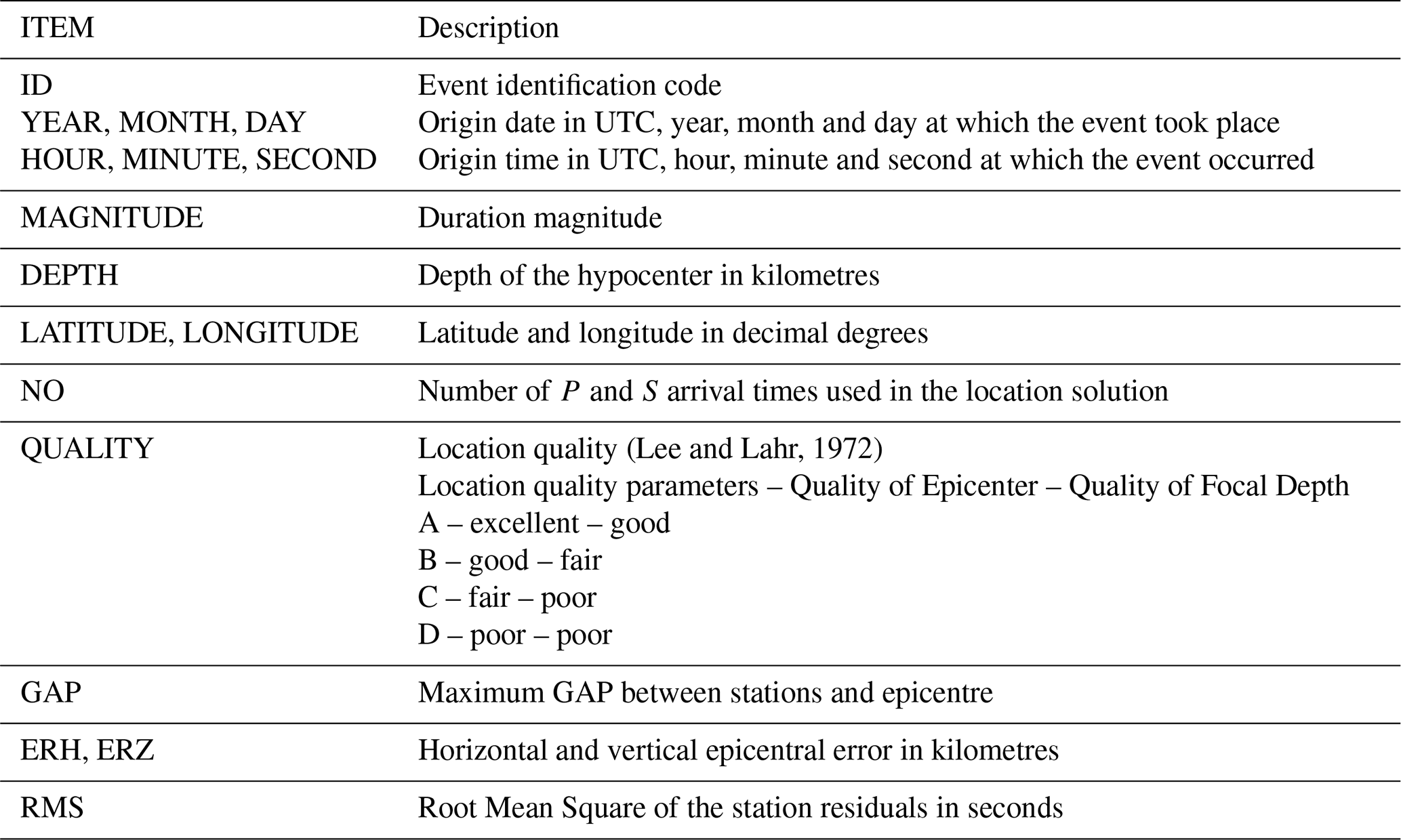
All the data were checked during the import phase in order to clean up any error and were projected into the UTM WGS84 reference system. The GeoDatabase is made up of a table of attributes whose items are summarized in Table 1. The GeoDatabase consists of 3064 VT earthquakes, 1517 of which were located by the Seismic Laboratory.

Table 1 Description of the GeoDatabase items.

The potential of the GeoDatabase resides in the easy management of data that can be quickly: displayed according to the information recorded in the items; selected with simple or complex queries; compared and correlated with other geographical information; used to generate new themes as a function of attributes or spatial distribution.

Two possible applications of GIS technology are illustrated below. First, we describe how to obtain a selection of a high quality dataset, necessary for any seismological analysis that requires reliable locations; as second application, we show how to identify and extract the swarms of CF. This last performance, described in Sect. 3, requires the use of the entire GeoDatabase (located and not located earthquakes), since it is based on the inter-arrival times of the earthquakes.

Figure 2 shows the high quality location of the VT earthquakes, selected according to location quality constraints. Such constraints were obtained through an empirical analysis, aimed at eliminating location artifacts (i.e., false epicenter alignments), possibly caused by problems in the convergence of the location algorithm (Lee and Lahr, 1972). The constraints are: location quality in the [A–C] interval, GAP ≤ 220^∘, and M_d ≥ 0.0. The selected 796 VT earthquakes in Fig. 2 are represented with a size proportional to their M_d values.

Maps similar to that of Fig. 2 are generated for monthly WEB reports on the areal distribution of the seismicity of Neapolitan volcanoes (http://www.ov.ingv.it/ov/bollettini-mensili-campania/BollettinoWeb_CF_dicembre2019.pdf, last access: 20 December 2020). The maps of the monthly WEB report are followed by evaluation/validation tests carried out by a focus group (teachers, geologists, architects) involved in the EDURISK project (http://www.edurisk.it, last access: 20 December 2020).

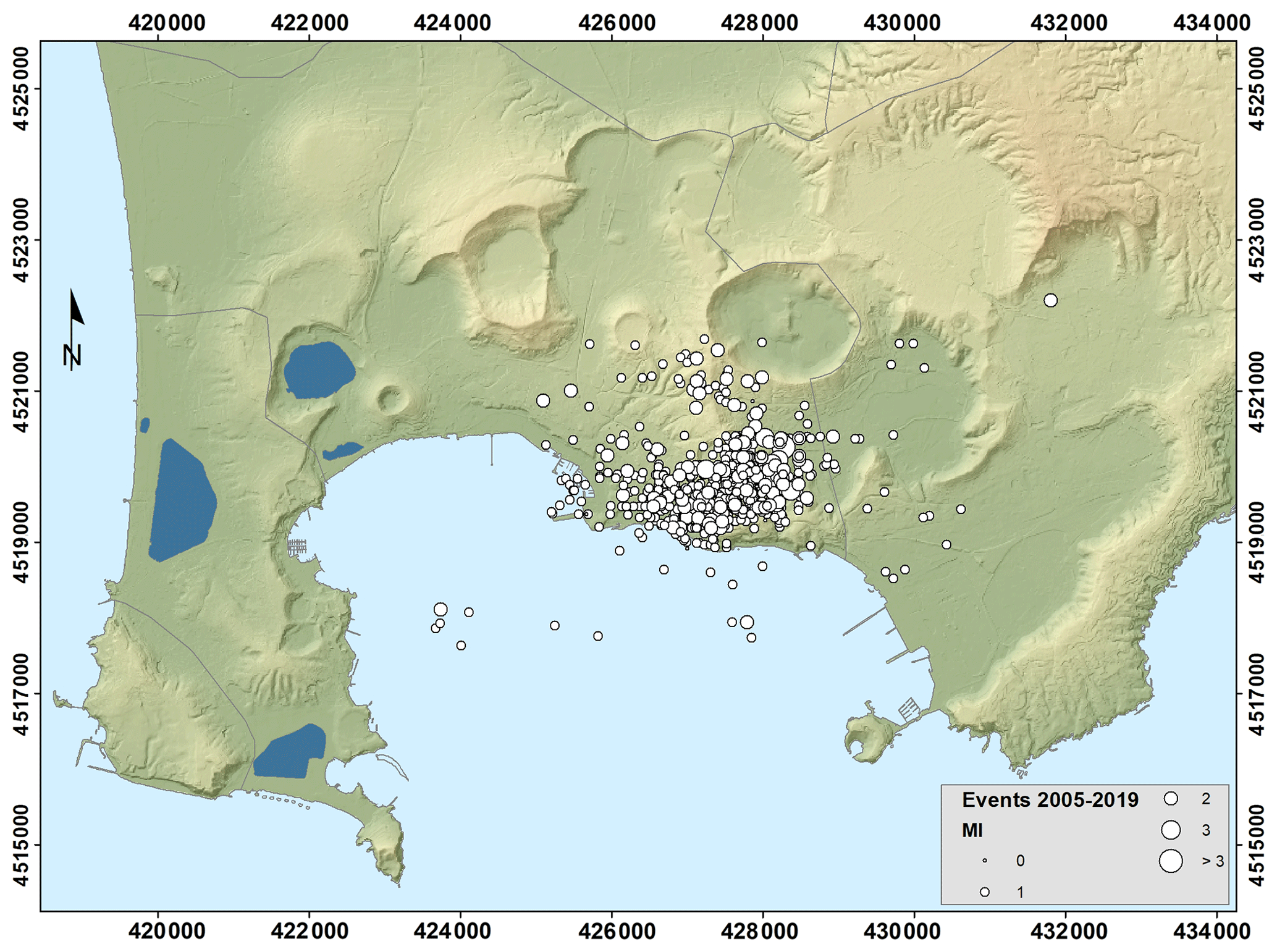
Figure 2 High quality VT earthquakes (see text) for the period 2005–2019. The size of the epicentres are shown as a function of the magnitude according to the legend on the bottom right. DTM of Campi Flegrei (Vilardo et al., 2013). Reference system UTM WGS84.

The distribution of VT earthquakes over time is shown in Fig. 3a. Despite the increase of the total number of VT earthquakes (both located and not), the percentage of not located VTs (N.L.), decreases over time respect to the total VT number. This decrease is explained by the increase number of installed seismic stations and by the improvement of both instruments (digital devices and broadband seismometers) and the quality of installation sites, which allows to identify and locate even very low magnitude events. The seismicity at CF is characterized by low M_d values (Aster and Meyer, 1988). Indeed, as shown in Fig. 3b, for 1729 earthquakes, the M_d value is less than 0 and only a single event has M_d greater than 2.5. For 393 VT earthquakes it was not possible to calculate M_d (N.C.) because of the low signal-to-noise ratio, or because they are superimposed to another VTs or to spurious transient signals, etc.

Figure 3 VT earthquake distributions: (a) Temporal distribution of located VT earthquakes and N.L. (left axis) and percentage of N.L. respect to all the VT earthquakes (right axis); (b) VT earthquakes distribution over M_d intervals.

Useful information can be obtained by analysing the pattern of the quality location parameters. In Fig. 4a the temporal distributions of the VT number associated to the location quality parameters are represented. It can be observed that the VTs with a better location (A, B and C) have increased in recent years, and the number of located VTs is greater than N.L. earthquakes. Observing M_d as a function of location quality (Fig. 4b), it is clear that as M_d decreases, the quality of location worsens or it is not possible to perform it. Furthermore, evaluating the trend over time of the GAP values (Fig. 4c), it is observed that both the maximum and minimum (max and min) values decrease over time. In the whole 2007 there was only one VT earthquake and, as a consequence, in the statistical calculation on the GeoDatabase, the max and min value of each parameter coincide for this year. Finally, the trend of the average RMS value (Fig. 4d) decreases over time.

In summary, for the data contained in the GeoDatabase all the described patterns indicate an improvement of the quality of the locations over the time, which follows the technological improvement of the instrumentation. Furthermore, as one expects, the higher the magnitude, the better the quality of the location.

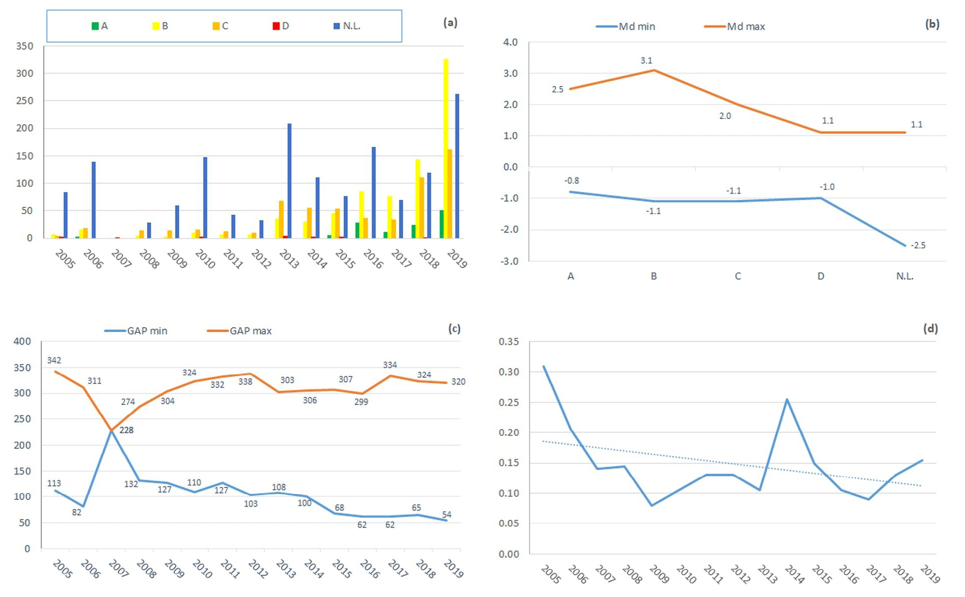
Figure 4 Location quality patterns. (a) VT earthquake time distribution for the location quality parameters (A, B, C and D) and time distribution of N.L. VTs; (b) Max and min M_d distribution over location quality parameters and N.L. category; (c) Max and min GAP distribution over time; (d) Mean RMS distribution over time (continuous blue line) and trend (dotted blue line).

3 CF swarms: Data analysis and results

As a second example of GIS application, we analysed the time distribution of all the earthquakes that occurred inside the CF caldera from 2005 to 2019, in order to understand the dynamics of the swarms with respect to the whole seismicity.

In order to identify the seismic swarms of CF, we used the operative definition inferred by the OV seismologists, which is used locally for the practical surveillance activities in agreement with the Italian CPD. This definition was obtained on the basis of the magnitude of the completeness for the CF seismic catalogue (http://www.ov.ingv.it/ov/it/banche-dati/186-cataloghi_sismici_vulcani_campani, last access: 20 December 2020) of the reference seismic station STH (M_d $=-\mathrm{1.0}$, Chiodini et al., 2017), the detection threshold (M_d = 0.5, Del Pezzo et al., 2013) and the statistical distribution of the VTs' inter-arrival times.

According to this definition, a seismic sequence is considered a CF swarm for surveillance scopes if at least 4 events occur in 30 min and at least 1 of them has M_d ≥ 0.0. Hereinafter, we will refer to a seismic sequence that meets the preceding definition as a CF-swarms. It is noteworthy that this definition serves to label a seismic sequence as a CF-swarm. In the following, when we refer to a CF-swarm we intend all the earthquakes that belong to the identified seismic sequence. We considered all the earthquakes in the GeoDatabase, regardless they are located or not, to analyse the temporal swarms' distribution in order to recover information on the hydrothermal/volcanic system (Chiodini et al., 2017; Petrosino et al. 2018). The GeoDatabase was mainly developed as a tool for surveillance purposes, within the interaction with CPD, that requires to account also for low magnitude earthquakes, regardless of the completeness threshold (M_d < −1.0). In addition, we will refer to the VT earthquakes that do not belong to CF-swarms as background seismicity.

By applying the statistical GIS tool Summarize, we created a table containing the daily number of VTs, together with the associated dates. It is noteworthy that in the observed period, on a total of 655 dates associated with occurrence of VT earthquakes, only 290 are associated with single VT. The remaining 365 dates contain more than 1 VT. In order to extract the CF-swarms, we used a query that counts all the seismic sequences that meet the requirements of M_d ≥ 0.0 (the created table contains also the max and min value of magnitude for a certain date) and an occurrence frequency ≥ 4, resulting in 157 dates. Over these 157 dates we performed a check over the time (hours, minutes, seconds and hundredths of seconds) to meet the criterion that at least 4 VTs occur in 30 min. We also considered the cases of CF-swarms occurring over two consecutive days. The dates that satisfy all the conditions were 113. Some properties of the obtained CF-swarms are reported in Fig. 5.

Figure 5 Some temporal properties of the CF-swarms extracted by GIS statistical tools between 2005 and 2019. (a) Distribution of the total number of VT earthquakes (blue) of each CF-swarm, and (b) Distribution over the time of the number of located VT earthquakes (red) of each CF-swarm. (c) max and min M_d, and (d) max and min depth b.s.l. of each CF-swarm.

Figure 6 shows the CF-swarms and the background seismicity occurred from 2005 to 2019, represented for four time intervals. Using the whole GeoDatabase for the selection of the CF swarms, the alignments with the grid bounds, linked to the poor quality of localization of small M_d earthquakes, are visible (see Sect. 2.2). In detail, in Fig. 6a the CF-swarms for the period 2005–2011, before the CPD decision to raise the alert level, are reported.

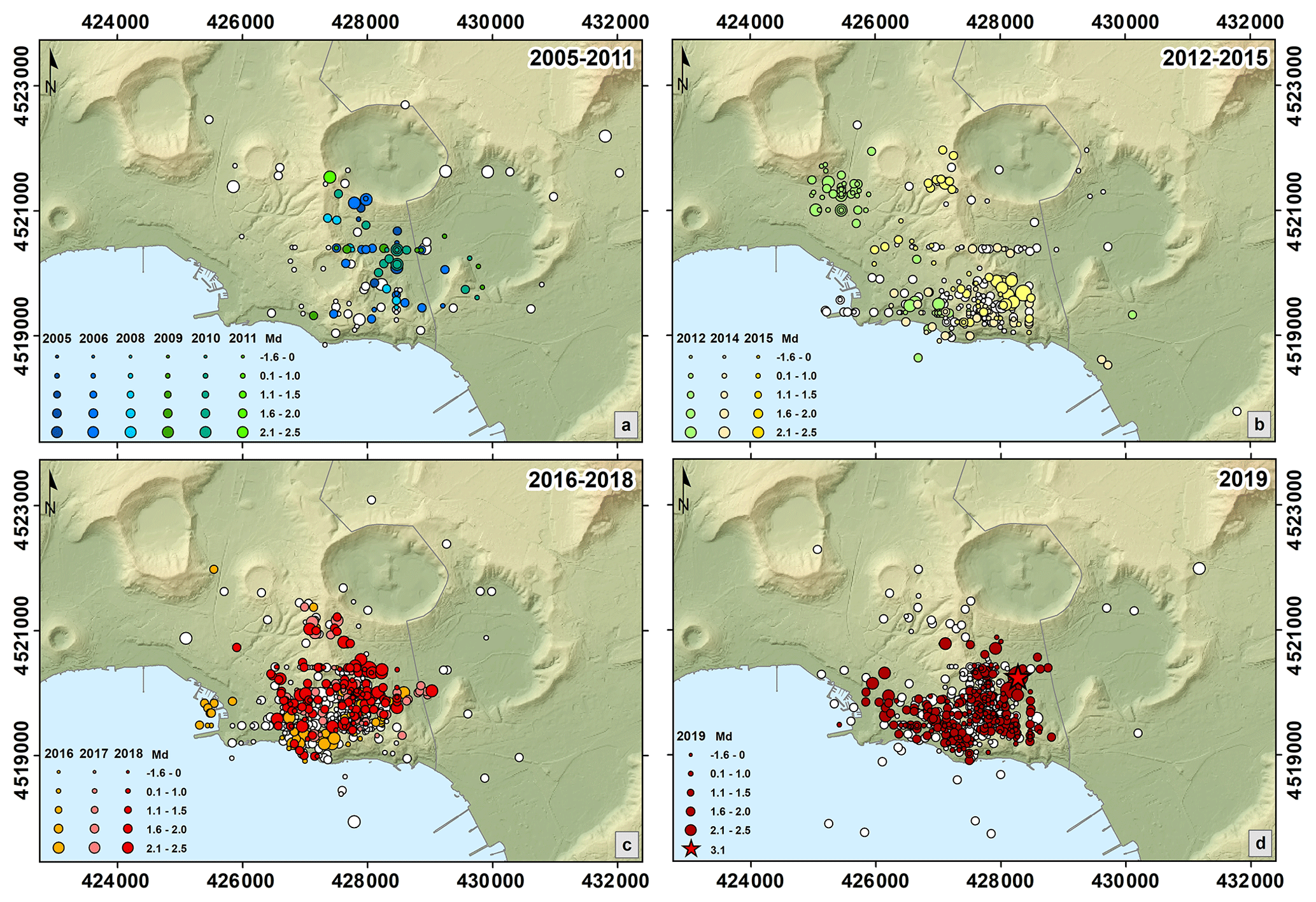
Figure 6 CF-swarms from 2005 to 2019: (a) from 2005 to 2011, (b) 2012–2015, (c) 2016–2018, and (d) 2019. The different symbols and sizes are used to indicate the year of occurrence and the magnitude value interval. The background seismicity of the related years is represented in white. DTM of Campi Flegrei (Vilardo et al., 2013). Reference system UTM WGS84.

In detail, in Fig. 6a the CF-swarms for the period 2005-2011, before the CPD decision to raise the alert level, are reported. As it can be seen, the swarms of that period have low magnitude values (M_d,max = 1.4) and are distributed in the northern, eastern and southern areas around Solfatara. The depths of these events are quite shallow, varying between 0.1 and 2.5 km (Fig. 5d). Starting from 2012 CF-swarms show an increase of the number of the CF-swarms (Fig. 6b) as well as the number of VTs, with a larger spatial distribution, denser towards the NW sector of Solfatara. An increment of the number of VTs and magnitude, which reaches a value of M= 2.5 on 7 October 2015 for the first time from the 1982–1984 crisis, was also observed. Only one deep earthquake occurred in 2012, with a depth of about 4 km b.s.l., while the remaining had a maximum depth that did not exceed 2.8 km. In the years 2016–2018 (Fig. 6c) the number of CF-swarms increases, with M_d = 2.4, and the density of the events, that concentrate inside Solfatara, Pisciarelli and the surroundings, grows up too. In these years, the maximum depth reaches 2.6 km. Finally in 2019 not only a net increase of all the seismicity (Fig. 6d), but also a rise of the number of CF-swarm is observed (Fig. 5a). The areal distribution of the VTs appears concentrated again in the south-western and eastern sectors surrounding Solfatara. During the last CF-swarm of 2019, on December 6th, the VT with the maximum magnitude M_d = 3.1 was recorded. In that year the swarms result shallower, with only three earthquakes that exceed 2 km of depth, reaching a maximum depth of 2.3 km. To better visualize how the CF-swarm hypocenters distribute with depth, in the Supplement we report the map and NS and EW vertical sections of the CF-swarms for each analysed year.

The CF-swarm increment and the occurrence rate in the last years do not correspond to an increase in the percentage of the number of CF-swarm VTs respect to all the VTs per year from 2005 to 2019. As it can be seen from Fig. 7, it is interesting to observe that until 2012 the most seismicity occurred in CF-swarms, with a percentage higher than 60 %, except for 2011 when the percentage is about 49 %. From 2014, the percentage remains around 50 %, varying from 44 % to 55 %, with a maximum of 65 % in 2014. In 2019, the percentage falls to 44 %, despite the remarkable increase of the total number of VTs and of the number of CF-swarms.

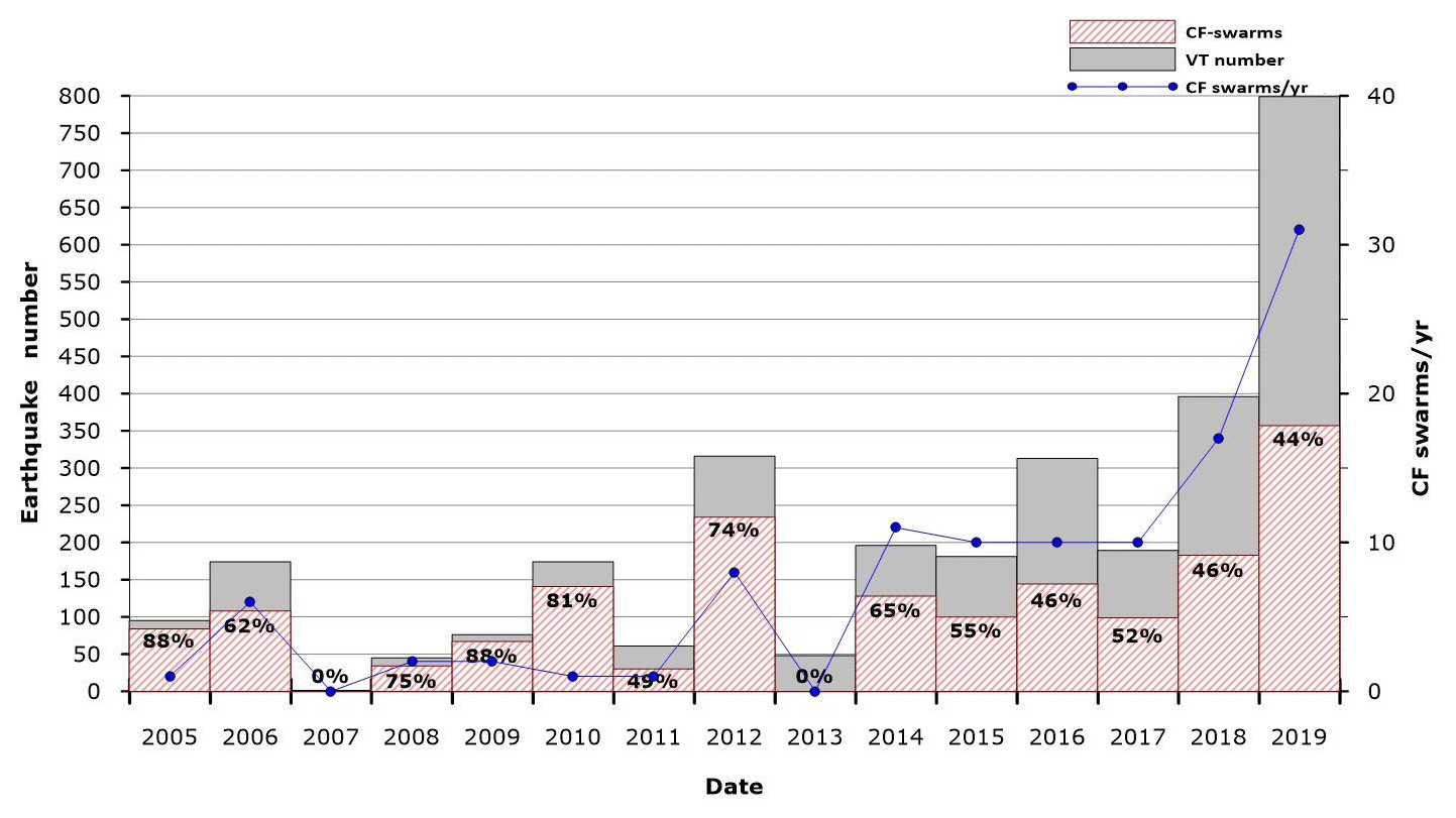
Figure 7 Annual distribution of all the VTs (gray), the VTs of the CF-swarm (red dashed), the number of CF-swarms per year (blue line) and the percentage of VTs of the CF-swarms respect to the number of all the VTs (percentage number) since 2005 to 2019.

In order to better compare the distribution of the CF-swarms with other kind of data (e.g. morphostructural, see Fig. 8), the maps of density per km² for the CF-swarms were produced by using GIS tools Point Density. This tool calculates the density of point features around each output raster cell. Conceptually, a neighbourhood is defined around each raster cell centre, and the number of points that fall within the neighbourhood is summed up and divided by the area of the neighbourhood (ESRI. ArcGIS Desktop, 2011). Results from this procedure are represented in Fig. 8, together with the morphostructural map of CF (Vilardo et al., 2013). This representation permits to relate the seismicity to the main tectonic lineaments of CF, which are represented by NW–SE, NE–SW and N–S striking faults.

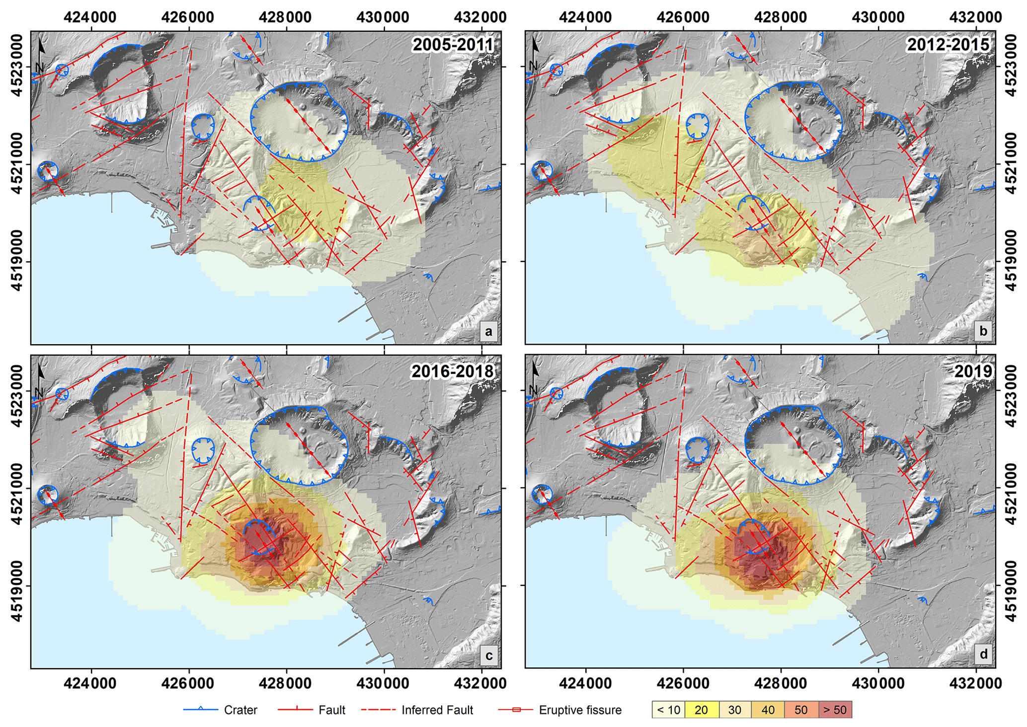
Figure 8 Density of CF-swarms from 2005 to 2019: (a) from 2005 to 2011, (b) 2012–2015, (c) 2016–2018, and (d) 2019. DTM and morphostructural map of Campi Flegrei (Vilardo et al., 2013). Reference system UTM WGS84.

Finally, we produced the seismic moment release maps by summing up the seismic moment of each VTs of the CF-swarms, for all the four time intervals, with the same grid of the density map. To calculate the seismic moment we used the equation retrieved from Galluzzo et al. (2004) for CF

$$\begin{array}{}\text{(1)}& \log M_{\mathrm{0}}=\mathrm{9.9}+\mathrm{0.9}{M}_{\mathrm{d}}\end{array}$$

where M₀ is the seismic moment expressed in Nm. We estimated the seismic moment release to give an idea of the actual energy release of the CF-swarms in the different years of analysis (Fig. 9). Both VT epicentral density and moment release maps indicate that most of the seismic energy is released at and around the Solfatara crater, which is also the area most involved in the recent uplift episodes.

Figure 9 Energy CF-swarms from 2005 to 2019: (a) from 2005 to 2011, (b) 2012–2015, (c) 2016–2018, and (d) 2019. DTM and morphostructural map of Campi Flegrei (Vilardo et al., 2013). Reference system UTM WGS84.

In particular, the density of the CF-swarms and the seismic moment distribution show a very similar spatial pattern for the years 2005–2011 and 2012–2015. The maximum values of density and seismic moment distribution for these years are respectively 16 and 25 earthquakes per km² and 13.7 and 59.9 × 10¹⁰ Nm. In the years 2016–2018, the density of CF-swarms increases to 60 earthquakes per km² and develops radially inside and to the west of the Solfatara. In the same period the seismic moment distribution increases up to a maximum of 80×10¹⁰ Nm, but remains within the same order of the previous periods. In 2019, the density of CF-swarms slightly decreases to 58 earthquakes per km², despite the fact that the total number of earthquakes is significantly higher than in previous years. The maximum density values are distributed within and in the south-southwest area around the Solfatara. The seismic moment distribution map instead shows peak values exceeding 10¹², which are distributed within a large area located northwest of the Solfatara Crater.

4 Discussion and conclusion remark

GIS are an important decision support tools and are used for territorial analyses in various fields and for disseminating any type of territorial information (Al-Dogom et al., 2018; Felpeto et al., 2007). In this study we presented two possible applications of GIS technology. First, we showed how to extract a high quality dataset on the base of location precision parameters. We assessed the reliability of the data (locations) through geostatistical analyses. In the second application, we considered all the earthquakes (located or not) of the GeoDatabase to individuate the CF-swarms and for highlighting their temporal trend over the last 15 years. The CF-swarms were identified through operative criteria, established to encounter volcanic surveillance requirements within INGV-CPD interaction. Concerning the definition of CF-swarms, it is noteworthy that it is not affected by the technological improvement to which the seismic network undergone through the time, since the network have a favourable spatial distribution since 2000. Moreover, CPD requires to account also for small earthquakes (M_d < 0.0).

The ability of the GIS to quickly select the VT earthquakes according to the desired classification criterion, allowed to perform statistical analyses on the CF-swarms (Fig. 5) and to represent them in different periods (Fig. 6). A better representation of these observations was possible thanks to the production of maps of the density of CF-swarms (Fig. 8). In this way it is possible to appreciate the greater density of VT earthquakes, information that could be lost in the traditional representation, because of symbols overlapping. Finally, a map of the distribution of the seismic moment was produced (Fig. 9).

The better readability of these maps allows to visually compare the trend of the CF-swarms with the morphostructural map and to hypothesize which structures are involved in the seismic activity. From 2005 to 2011, most of the seismicity occur in CF-swarms with a maximum M_d of 2.0 (Fig. 5c) and a maximum depth of approximately 2.5 km (Fig. 5d). The CF-swarms are distributed in the northern, eastern and southern areas around the Solfatara, affecting the NW-SE and NE-SW faults of the Solfatara, as evidenced by the CF-swarms density map (Figs. 6a and 8a). The distribution of the seismic moment show a spatial trend very similar to the CF-swarms density map (Fig. 9a). According to Di Luccio et al. (2015) and Petrosino et al. (2018), the CF-swarms in this period appear to be related to the hydrothermal activity of the area.

In the period 2012–2015, some CF-swarms shear the same source volume as the seismicity of 2005–2011, in the Solfatara-Pisciarelli area. Furthermore, in 2012 a significant number of the VTs is located between the Gauro and Cigliano (Figs. 1, 6b and 8b), where the NS-striking faults to the West of the Solfatara seem to be involved. The depth of these CF-swarms varies between 3 and 4 km in 2012, and then becomes shallower until the end of 2015 (Fig. 5d). The CF-swarm that occurred in 2012 (with a VT earthquake of M_d,max = 2.5, Fig. 5c) is associated with fractures, due to the release of gas from a localized magma body and/or a volumetric increase in this body (Di Luccio et al., 2015).

Since 2016, the number of VT earthquakes has gradually increased, while the percentage of CF-swarms remains fairly constant and the occurrence frequency decreases (Fig. 7); the depth of the CF-swarms is again low (0–3 km) (Fig. 5d). In this period, the VT earthquakes are concentrated in proximity of the NW-SE and NE-SW fault systems, in the area between Solfatara and Pisciarelli (Figs. 6c and 8c). The M_d of earthquakes does not significantly increase (Fig. 5c), while the distribution of the seismic moment increases in this area (Fig. 9c).

The increase in background seismicity, which began in 2015, reaches its peak in 2019, while the number of CF-swarms decreases (Fig. 7). The depth of the CF-swarms becomes shallower (maximum depth = 2.8, Fig. 5d). It should also be noted that the NW-SE and NE-SW faults of the Solfatara are always involved (Figs. 6d and 8d), but the epicentral distribution and the seismic moment release show a different shape, with the higher moment release values at north-west of the Solfatara (Fig. 9d). In fact, by carefully observing the symbolism of M_d in Fig. 6d, it is evident that in this area the earthquakes with the highest M_d occurred.

Among all the observations made, a very interesting scientific result stands up. As it can be observed in Fig. 7, the increase in seismic activity of CF does not always correspond to an increase in CF-swarms, but in the last years of observation a significant increase in background seismicity was observed. To further investigate this phenomenon, we evaluated the inter-arrival time of VT earthquakes of the CF GeoDatabase. The split times between the earthquakes were calculated using the non-declusterized catalogue (swarms and background), applying different magnitude thresholds (M_d > 0.5, M_d > 0.0, M_d > −0.5, and M_d > −1.0). The distributions of the inter-arrival times in the period 2005–2019 shows a bimodal distribution (Fig. 10) likely due to the presence of both seismic swarms and background seismicity. These distributions show a very good match with the inter-arrival times estimated by Chiodini et al. (2017). Since those authors used the VTs from 2000 to 2016, our analysis could be considered as the continuation/confirmation of their study.

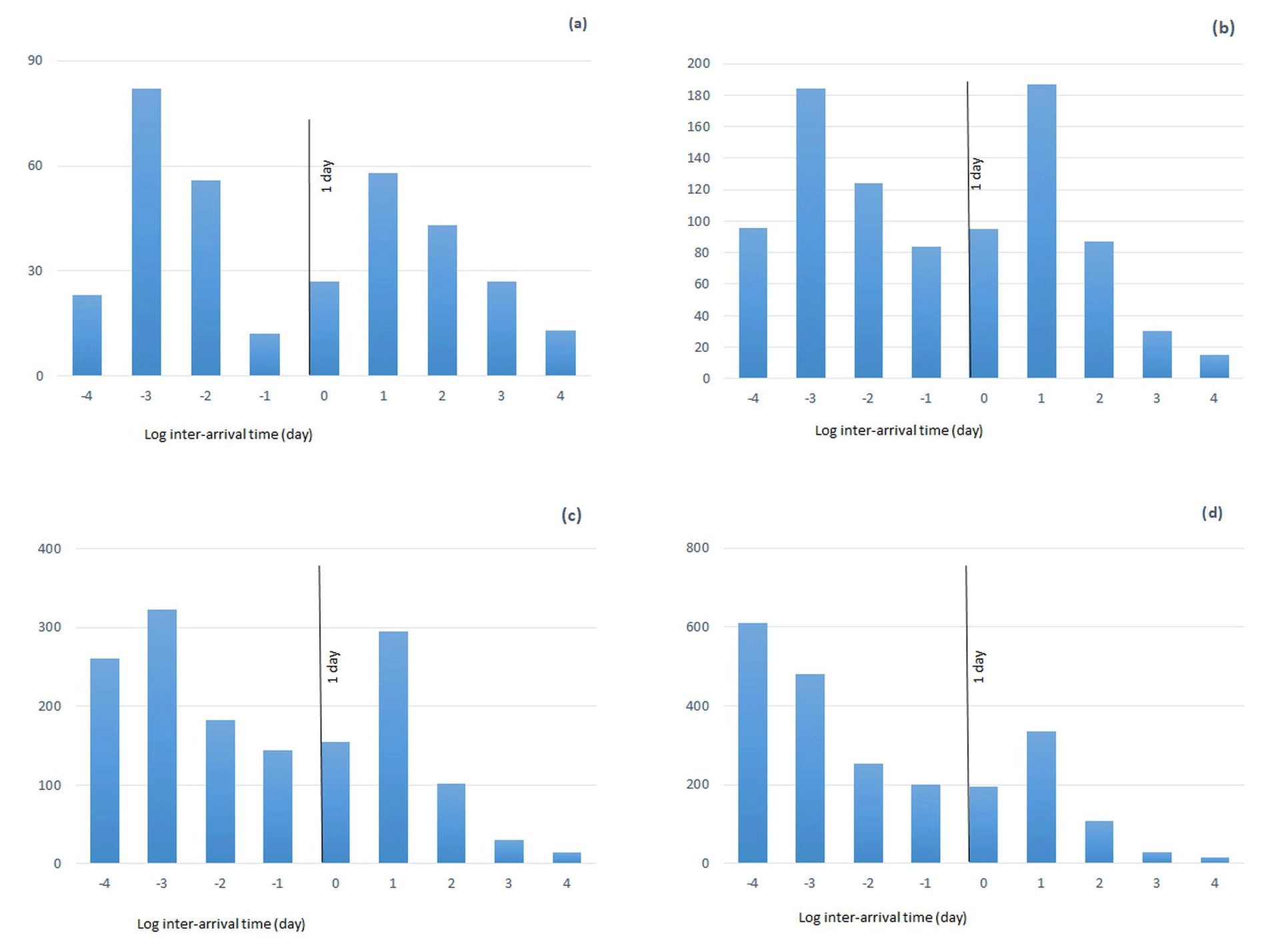
Figure 10 Histograms of the log inter-arrival time of CF VTs: (a) for M_d > 0.5, (b) for M_d > 0.0, (c) for M_d > −0.5, and (d) for M_d > −1.0.

The increase of background seismicity against a decrease of CF-swarms was also noted by Petrosino et al. (2018) for the earthquakes in the period 2005–2016. Those authors indicate that this type of seismicity was mostly influenced by external factors (rains, crustal tides) and had strong characteristics of periodicity, until the end of 2012. Chiodini at al. (2017), attribute the variation in the observed seismicity pattern to a gradual transition from the fragile to the plastic behaviour of rocks associated with very high temperatures, caused by multiple magmatic fluid injections. Petrosino et al. (2018) invoke a passive degassing mechanism, from a magma standing at a certain depth and losing volatiles by diffusion and/or exsolution due to oversaturation. Without entering into such debate, we stress that the integration and rapid analysis of multidisciplinary data sets via GIS technologies may provide fundamental contributions to any study on the origin and nature of seismicity at the CF.

In conclusion, all the observations made in the present work were quickly retrieved thanks to fast operations and analyses in GIS environment. All the described analyses can be readily repeated in case it should be necessary to change the criteria for the CF-swarm definition. Moreover, the possibility of quickly visualize the information, according to different representation criteria, permits to highlight complex behaviors. Finally, having other spatial information, such as active faults, settings of past deposits, acting deformations, etc., GIS may allow to represent and to correlate these information, thus leading to better understanding of the acting dynamics. In conclusion, GIS represent an indispensable supporting tool to decision in volcanic unrest.