A three-dimensional lithospheric-scale thermal model of Germany

We present a 3-D lithospheric-scale model covering the area of Germany that images the regional characteristics of the structural configuration and of the thermal field. The structural model resolves major sedimentary, crustal and lithospheric mantle units integrated from previous studies of the Central European Basin System, the Upper Rhine Graben and the Molasse Basin, together with published geological and geophysical data. A combined workflow consisting of 3-D structural, gravity and thermal modelling is applied to derive the 3-D thermal configuration. The modelled temperature distribution is highly variable in response to an imposed heterogeneous distribution of thermal properties assigned to the different units. First order variations in the temperature field are mainly attributed to the thermal blanketing effect from the sedimentary cover, the variability in the amount of radiogenic heat produced within the different crystalline crust compartments and the implemented topology of the thermal Lithosphere-Asthenosphere Boundary.

1 Introduction

Being a key topic for the present-day scientific and industrial community, the global climate change leaves us no choice but developing a strategy of provision of renewable energy resources, such as geothermal. Geothermal energy is transported by conduction and convection from deeper parts of the earth towards the surface and can be extracted by geothermal power and heating plants from natural and/or engineered reservoirs. Using such energy requires knowing the temperature distribution in the light of the causative processes, the latter being influenced by the tectonic, geological and hydrogeological setting of the target area. Knowledge about reservoir's temperatures can be obtained directly by costly drilling, that only provides local information on temperature at a specific depth without any knowledge of the relevant physical processes. For regional exploration, complementary workflows use integrated 3-D structural and physics-based models that help to predict the temperature distribution in the subsurface by taking into account the heterogeneous structural configuration as well as the, often non-linear, causative processes (e.g. Cacace et al., 2010; Scheck-Wenderoth et al., 2014).

Though several regional models have focussed on different regions of Germany (Sippel et al., 2013; Scheck-Wenderoth et al., 2014; Przybycin et al., 2015; Freymark et al., 2017), a consistent subsurface structural and thermal model for the whole territory of Germany is still missing. Here, we integrate all available information of these studies into a consistent 3-D model of Germany referred to as 3-D-Deutschland (3-D-D) hereafter, that provides the background to be further used in future regional-to-local investigations. Therefore we integrate three regional structural models based on data comprising borehole measurements, seismic profiles, isopach and geological maps and constrained by gravity and thermal data (Fig. 1): (1) the Central European Basin System (CEBS, Maystrenko and Scheck-Wenderoth, 2013), (2) the Molasse Basin (MOLA, Przybycin et al., 2014) and (3) the Upper Rhine Graben (URG, Freymark et al., 2017).

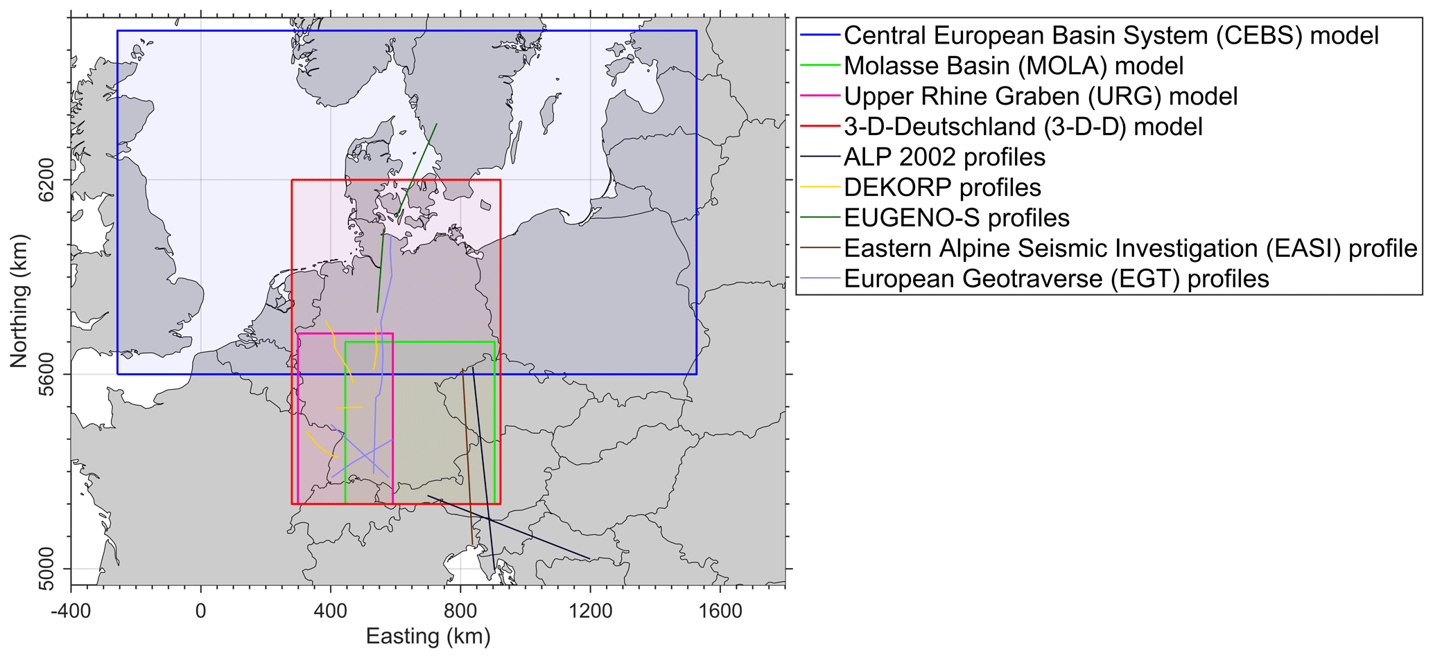
Figure 1 Geographical map of the regional model boundaries and seismic profiles used to solve discrepancies. The 3-D-D model area is shown in red and spans 1000 km in North-South and 643 km in East-West direction. Map coordinates in this and in all following figures are given in km in UTM Zone 32N coordinate system.

2 Methods

The applied workflow comprises (1) structural modelling to correlate the lithostratigraphic units derived from the different input models, followed by (2) a validation of the derived configuration with 3-D gravity modelling and, lastly, (3) the calculation of the conductive thermal field. The main challenge in joining the three existing models was to identify layers of corresponding lithostratigraphy and to merge these for the whole 3-D-D model area (Fig. 1, Table 1). Therefore, we revisited published seismological data to overcome inconsistencies across the boundaries of the input models.

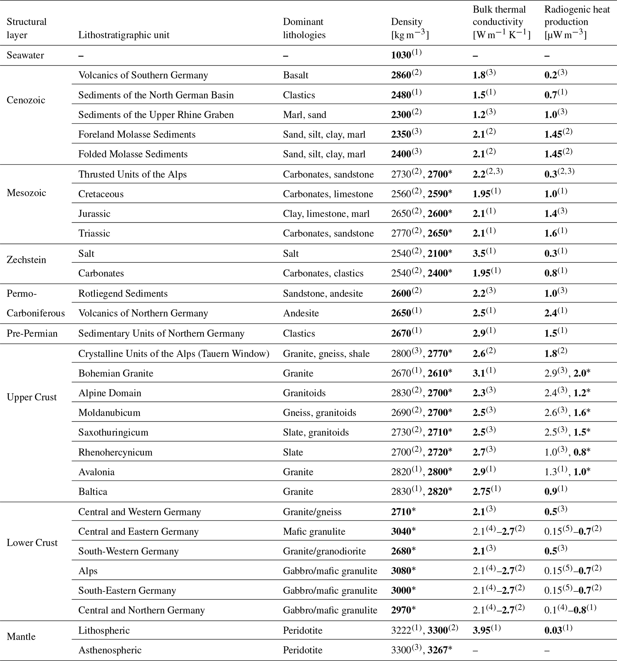
Table 1 Dominant lithologies, densities and thermal properties assigned to layers of the 3-D-D model for gravity and conductive thermal steady-state calculations: (1) Scheck-Wenderoth et al. (2014); (2) Przybycin et al. (2015); (3) Freymark et al. (2017); (4) Norden et al. (2008); (5) Vilà et al. (2010). Final validated parameter values are marked bold; (*) stars indicate values adjusted in response to the 3-D effects of the larger volumes of certain units in the 3-D-D model compared to the input models.

2.1 Structural modelling

2.1.1 Input data

The data used for this study include the ETOPO1 Global Relief Model (Amante and Eakins, 2009), the configurations of the three regional models and the seismic profiles of the deep seismic experiments EUGENO-S (EUGENO-S Working Group, 1988), the DEKORP (e.g. Meissner and Bortfeld, 2014), the EGT (Blundell et al., 1992) and the ALP2002 (Brückl et al., 2007). These profiles helped to constrain the structural configurations across the boundaries of the regional models (Fig. 1). For the gravity modelling stage we rely on the global combined reference gravity field model EIGEN-6C4 (Förste et al., 2014; Ince et al., 2019). Geological depth maps (Bayrisches Staatsministerium für Wirtschaft, 2004) and thickness maps of Boigk and Schöneich (1974) were also used to correlate boundaries of the Triassic across the three models (Lechel, 2017). Results of the Eastern Alpine Seismic Investigation (EASI) project (Hetényi et al., 2018) were integrated to refine the Mohorovičić discontinuity (Moho) in the SE part (Fig. 1) of the model. To derive a consistent Lithosphere-Asthenosphere boundary (LAB) we integrated results from the three input models, validating the interpolated boundary with lithospheric thicknesses derived from receiver functions data (Geissler et al., 2010).

The Central European Basin System (CEBS) model integrates geological and well data, deep seismic experiments (e.g. DEKORP-BASIN'96: Bleibinhaus et al., 1999; EUGENO-S: EUGENO-S Working Group, 1988; EGT: Blundell et al., 1992), magnetic and magnetotelluric studies and gravity modelling (see Maystrenko and Scheck-Wenderoth, 2013 for an overview). The model covers Northern Central and Western Europe (Fig. 1) and has a grid resolution of 4 km (Maystrenko et al., 2013). The CEBS model contains up to 12 km of Permian to Cenozoic deposits resolved as eight different stratigraphic units, two different units of the upper crystalline crust, a lower crustal unit and the lithospheric mantle.

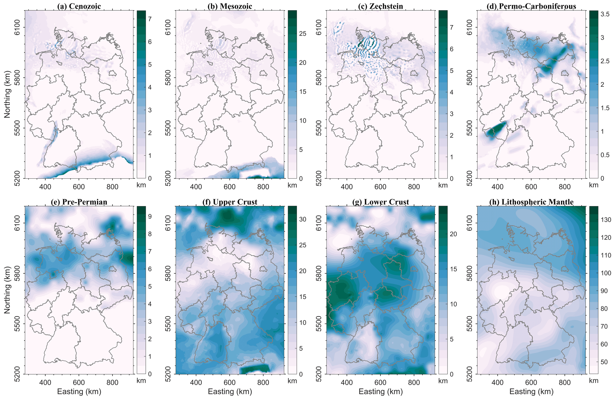
Figure 2 Thicknesses of the major structural layers of the 3-D-D model: (a) Cenozoic; (b) Mesozoic; (c) Zechstein; (d) Permo-Carboniferous; (e) Pre-Permian; (f) Upper Crust; (g) Lower Crust; (h) Lithospheric Mantle. Colour bars show thickness in km.

The Molasse Basin (MOLA) model, with a grid resolution of 2.5 km, includes the northern portion of the Eastern Alps and extends over SE Germany, Western Czech Republic and Western Austria (Fig. 1). The stratigraphic subdivision of the model resolves Cenozoic to Upper Jurassic Sediments, the impact structure of the Nördlinger Ries, a geological unit of the Alpine nappes, an upper and a lower crystalline crust and a uniform lithospheric mantle (Przybycin et al., 2014, 2015). The model is consistent with seismic experiments (e.g. TRANSALP, Gebrande, 2001; ALP2002, Brückl et al., 2007; ALPASS, Mitterbauer et al., 2011, well logs, local models and geological atlas data (see Przybycin et al., 2014 for an overview).

The Upper Rhine Graben (URG) model likewise integrates results from many studies (see Freymark et al., 2017 for an overview) such as seismic surveys, (e.g. DEKORP: Meissner and Bortfeld, 2014; KTB: Lüschen et al., 1989; EGT: Blundell et al., 1992), 2-D gravity modelling (Campos-Enriquez et al., 1992), regional studies of the GeORG and EUCOR-URGENT projects (Behrmann et al., 2005; GeORG-Projektteam, 2013), or borehole measurements. The URG model covers SW Germany, NE France and Northern Switzerland (Fig. 1) and has the finest grid resolution of 1 km (Freymark et al., 2017). It resolves seven lithostratigraphic units including different lithologies of the Cenozoic and Mesozoic as well as different lithostratigraphic units of the Alps. The upper crystalline crust is differentiated into different Variscan structural domains overlying a lower crystalline crust and two units of the lithospheric mantle.

2.1.2 3-D structural and gravity modelling

Consistent merging of the stratigraphic surfaces of the original input models proved to be a non-trivial task due to the differing resolution and related uncertainties of the marginal domains caused by insufficient data coverage. In order to resolve geometric conflicts among the three models and to integrate additional available data, all surface grids of the original models were first correlated according to their lithostratigraphic sequences and then loaded into Petrel. Discrepancies between the units were removed by revisiting seismic profiles across the boundaries of the regional models (see Sect. 2.1.1; Fig. 1). After integration, data for each unit were interpolated using the convergent interpolation algorithm of Petrel into a regular grid with 1 km spacing (Lechel, 2017). 3-D gravity modelling was carried out using IGMAS+ (Götze and Lahmeyer, 1988; Schmidt et al., 2010), an interactive software for 3-D gravity and magnetic modelling. The interpolated surface grids bounding the resolved geological units were imported to IGMAS+ to build a 3-D density model, produce its gravity response and adjust densities (see Table 1) to fit the response to the gravity disturbance computed for EIGEN-6C4 gravity model at 6 km height (Förste et al., 2014).

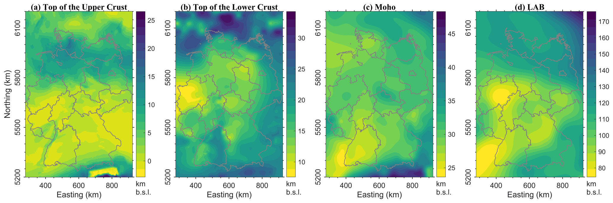
Figure 3 Thicknesses of the major structural layers of the 3-D-D model: (a) Cenozoic; (b) Mesozoic; (c) Zechstein; (d) Permo-Carboniferous; (e) Pre-Permian; (f) Upper Crust; (g) Lower Crust; (h) Lithospheric Mantle. Colour bars show thickness in km .

2.2 Conductive thermal modelling

To assess the distribution of deep temperatures resulting from the structural configuration of the 3-D-D model, we calculate the present day conductive thermal field under steady-state conditions. For that purpose we use GOLEM (Jacquey and Cacace, 2017; Cacace and Jacquey, 2017) – a 3-D thermal-hydraulic-mechanical simulator based on a Galerkin finite-element technique. Consistently with all previous studies (Scheck-Wenderoth et al., 2014; Przybycin et al., 2015; Freymark et al., 2017), we assign uniform lithology-dependent thermal properties to each resolved stratigraphic unit (Table 1). As an upper boundary condition we consider the spatially variable annual average surface temperature (DWD, 2019) onshore, together with constant 4 ^∘C at the seafloor. The thermal LAB with constant 1300 ^∘C (Turcotte and Schubert, 2002) represents the lower boundary condition.

3 Results and discussion

3.1 3-D structural setting

The resulting 3-D-D model comprises 31 lithostratigraphic units (Table 1): seawater, 14 sedimentary units, 14 crystalline crustal units and 2 lithospheric mantle units. The thicknesses of cumulative sedimentary, crustal and mantle layers are shown in Fig. 2a–d.

The top surface of the Cenozoic sediments layer is constrained by the topography onshore and bathymetry offshore. The layer encompasses volcanic rocks (distinguished only in the SW of Germany, Lechel, 2017) and sedimentary rocks spatially subdivided into the North German Basin, the Upper Rhine Graben and the Molasse Basin. The Cenozoic layer reaches up to 7 km of cumulative thickness in the Molasse Basin, but is absent or thin in the Alps, Central and NE Germany (Fig. 2a).

The Mesozoic sedimentary layer comprises the Thrusted Units of the Alps (Helvetic and Austroalpine nappes), as well as Cretaceous, Jurassic and Triassic sediments. The Thrusted Units of the Alps are dissected in the Tauern Window where metamorphic and crystalline upper crustal rocks crop out (Fig. 2b). Cretaceous sediments occur mainly in the North German Basin. Jurassic sediments are present in Northern Germany and beneath the URG, as well as in Southern Germany along the present-day mountain ranges of the France-Swiss, the Swabian and the Franconian Jura. The Triassic unit is represented as “Germanic Triassic” (Alpine Triassic is already integrated as the Thrusted Units). The cumulative thickness of the Mesozoic layer reaches 30 km in Alps and 10 km in Northern Germany (Fig. 2b), where it has an irregular structure due to widespread salt tectonics. The latter is related to postdepositional mobilisation of the Upper Permian Zechstein evaporites (Maystrenko et al., 2013) located mainly in the North German Basin with an average thickness of 1.0 to 1.5 km and classified into carbonates and rock salt, considering variation in facies. Locally the Zechstein Salt thickness reaches up to 8 km in locations where salt diapirs and walls pierce their Mesozoic and Cenozoic cover (Fig. 2c). The Zechstein Carbonates at the margins of the Zechstein Basin reach up to 1.1 km and pinch out southwards in the Hesse Depression and the URG (Lechel, 2017).

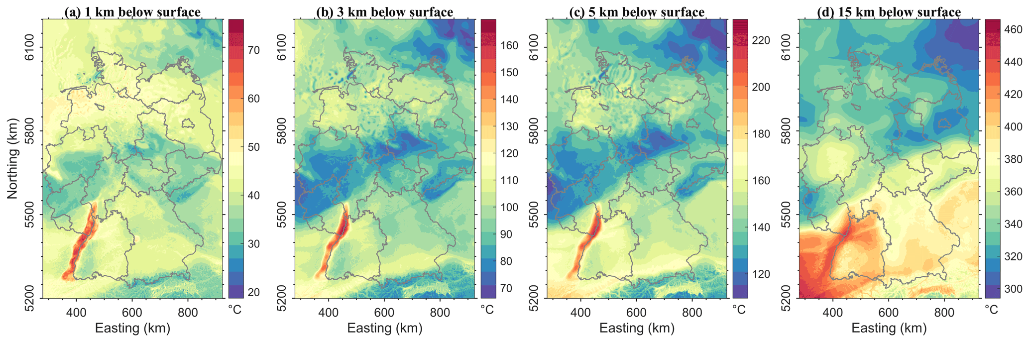
Figure 4 Modelled temperatures at: (a) 1 km; (b) 3 km; (c) 5 km; (d) 15 km depth below surface. Colour bars show temperature in ^∘C.

Figure 5 Depths of the isotherms: (a) 60 ^∘C; (b) 100 ^∘C; (c) 450 ^∘C and (d) 600 ^∘C. Colour bars show depth in km below earth's surface.

The next-deeper major layer, the Permo-Carboniferous (Fig. 2d), comprises the units of the Lower Permian Rotliegend sediments and the Permo-Carboniferous volcanics. The Rotliegend sediments are up to 2.3 km thick in the North German Basin, and scattered in Thuringia, Hesse, NW Bavaria and Northern Baden-Württemberg, reaching a thickness of up to 3.5 km in the Saar–Nahe Basin (Fig. 2d). The Permo-Carboniferous volcanics are present both in Northern and Southern Germany but only relevant in the northern part with more than 2.6 km thickness (Fig. 2d).

The Pre-Permian layer consists of partly metamorphosed Palaeozoic sediments deposited before and during the Variscan Orogeny. This layer could only be differentiated from the crystalline Upper Crust below Northern Germany, where it is wide-spread, having a thickness of about 4.0 km in average and reaching 9.5 km in the north-eastern part of the model (Fig. 2e). At the northern mountain ranges of the Harz, the Ore Mountains and the Rhenish Massif, the layer crops out while it lies between 5 and 12 km deep below the North German Basin (Lechel, 2017).

The Upper Crust unit was differentiated into domains with similar lithologies according to their orogenic origin (Alpine, Moldanubian, Saxothuringian, Rhenohercynian, Baltic Shield). It also comprises local units of the Bohemian Granites and the Tauern Body (Table 1). Therefore, the Variscan domains defined in the URG model (Freymark et al., 2017) were extended to the whole 3-D-D model according to the classification of Pharaoh (1999). The Upper crystalline Crust crops out in the Bohemian Massif, the Vosges and the Black Forrest (Fig. 3a) and attains an average cumulative thickness of 17 km (Fig. 2f). Below the Baltic Shield and Saxony, as well as in the area of the Tauern Body, the Upper Crust is the thickest (up to 32 km), whereas the thinnest Upper Crust is below the North German Basin and the Rhenish Massif, locally less than 2.0 km (Fig. 2f).

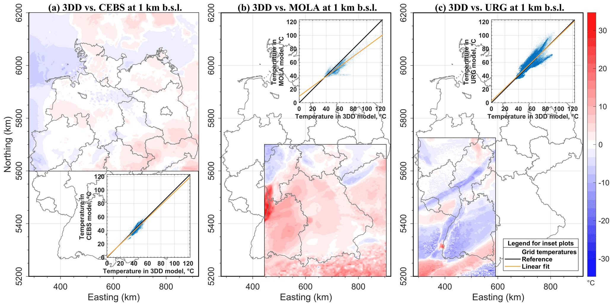
Figure 6 Comparison of thermal field of 3-D-D model at 1 km b.s.l. with (a) CEBS, (b) MOLA, (c) URG in corresponding areas. Colour bar show temperature difference in ^∘C scaled equally in all three panels. Each panel is complemented with a cross-plot of grid temperature values and their linear fit.

The thickness of the Lower Crust unit is about 12 km in average. It reaches 24 km under the Rhenish Massif and the part of the CEBS where the Upper Crust thins out (Fig. 2f–g). Below some parts of the Netherlands, Denmark and the Ore Mountains the Lower Crust is absent (Fig. 2g). There the thick Upper Crust is characterized by low P-wave velocities (<6.5 km s⁻¹) and densities (<2850 kg m⁻³) and thickens south of the Elbe Line. The top of the Lower Crust deepens to 34 km below Denmark and reaches its shallowest point below the Rhenish Massif and the Ardennes with 7 km b.s.l. (Fig. 3b).

The Lithospheric Mantle is considered as peridotites constrained by the Moho at the top (Fig. 3c) and the LAB at the bottom (Fig. 3d). It has an average thickness of 77 km with a minimum of 43 km below the Western part of Germany and a maximum of 138 km below the Baltic Shield (Fig. 2h). The Moho surface (Fig. 3c) was integrated from the input models and adjusted in the SE part using the EASI Moho profile (Hetényi et al., 2018). The lowermost surface of the model, the LAB, represents a varying topology across Germany between 74 and 176 km depth with a mean value of 108 km (Fig. 3d). The Lithospheric Mantle is deepest and thickest under the Baltic Shield (Figs. 2h, 3d).

3.2 Temperature distribution

The predicted temperatures vary in response to the heterogeneous distribution of the thermal properties associated with the different lithological units (Table 1). The highest shallow temperatures (Fig. 4a–d) are predicted within the Upper Rhine Graben, though elevated shallow temperatures are also modelled for the CEBS and the Molasse Basin. The coldest shallow domains are predicted in areas where the crystalline crust crops out or is close to the surface. Thus the short-wavelength variations of shallow temperatures are mainly influenced by the blanketing effect of a less conductive sediments compared to a more conductive crystalline rocks or rock salt. The modelled surface heat flow varies in the range of 60–100 mW m⁻² in concordance with several published reference maps (Majorowicz and Wybraniec, 2011; Norden et al., 2008; Fuchs and Balling, 2016).

Accordingly, temperatures of 100 ^∘C (usually targeted by geothermal industry, see e.g. DiPippo, 2012), are reached at 1.5 km below surface in the URG (Fig. 5b), but the depth of this isotherm can be up to 4.5 km below surface in areas of shallow crystalline crust. The thermal pattern changes with depth: the wavelength of temperature variations increases as indicated by widening of areas of elevated temperatures. This variation is due to the superposed additional influence of the volume distribution of radiogenic heat produced by felsic upper crystalline crust (Variscan and Alpine domains) and the depth of the thermal LAB. Therefore, hotter deep temperatures correlate with locations where the upper crust is thicker and the LAB is shallower as illustrated by the isotherm depth maps (Fig. 5a–d).

3.3 Comparison of thermal models

In order to quantify the consistency of the newly derived 3-D-D model with the three input models (that were properly validated with measured temperatures) we analysed the temperature differences at 1 km b.s.l (Fig. 6a–c). The models are consistent concerning the regional pattern and the range of temperature variations. The higher misfits (up to 30 ^∘C) along the boundaries of the input models are related to decreasing data coverage of the input models towards their margins (this also caused structural inconsistencies explained in Sect. 2.1). Therefore, the joint 3-D-D model naturally predicts different temperatures in these overlapping domains. Another discrepancy is related to the stratigraphic resolution that is higher in the input models (especially in URG model, Fig. 6c), this also naturally results in different predicted temperatures. Finally, the three input models used different upper boundary conditions in their thermal simulation. In general, the 3-D-D model is mostly consistent with the CEBS model, slightly colder than the URG model (due to lower stratigraphic resolution) and hotter than the MOLA model (Fig. 6a–c).

Cross-plots of the temperature values in the coinciding grid nodes together with their linear fit (inset plots in Fig. 6a–c) reveal that the most of the discrepancies are found for the MOLA model, mainly in the Alpine area and along the boundary with the URG model (Fig. 6b). In the CEBS part (Fig. 6a) main discrepancies are on the margins of the area and can be explained by a smaller extent of the 3-D-D model (Fig. 1) leading, e.g. to the lack of thermal impact from the unconsidered shallow LAB in the NW part of the larger CEBS model (Maystrenko and Scheck-Wenderoth, 2013). Discrepancies in the URG area form two linear trends in the cross-plot (inset plot in Fig. 6c) corresponding to the areas of negative and positive temperature misfit, although the linear fit is the best of all three models. A proper comparison to the results of the statistical interpolation of measured temperatures by Agemar et al. (2012) would be beneficial, however these measured temperatures are not freely available and the temperature profiles in Agemar et al. (2012) don't display calibration wells. Moreover, there is a high probability that interpolation over salt structures predicts wrong temperature distributions: temperatures from wells penetrating the salt show a far larger chimney effect, which was nicely demonstrated by Fuchs and Balling (2016). Therefore, model validation is possible only in terms of regional pattern of subsurface temperature variations and ranges of temperatures at certain depths, while a more detailed calibration would require local models of higher structural resolution that consider also the effects of coupled heat and fluid transport.

3.4 Model limitations

It is clear that the derived model is built on assumptions that introduce uncertainties. First of all, the assumption of steady state may not be valid and neglecting the effects of previous glaciations or rifting phases would over- or underestimate shallow temperatures. Sensitivity studies have shown that such effects would influence the absolute values of temperatures but not their regional distribution pattern (Majorowicz and Wybraniec, 2011). Neglecting the influence of coupled fluid and heat transport may also lead to erroneous conclusions as the conductive thermal model that best reproduces the observed heat flow considers an “effective” thermal conductivity that contains the superposed effects of different heat transport processes (Cacace et al., 2010). Again, local studies would be required to better quantify the absolute impact of this simplification. The quality and quantity of observations decreases with depth. The indirect methods of deriving the depth to the thermal LAB come with their own limitations and future improvement would require more densely spaced passive seismic experiments. Comparing the results for our model with seismically constrained LAB and a model with the LAB assumed at a constant depth of 120 km, we estimated the impact on temperature variations in the upper 3 km in the range of ±25 ^∘C. Finally, assuming laterally homogenous thermal properties in the different model units is an additional approximation. Improvement here would require either validation by densely-spaced measurements of rock properties in outcrop analogues or in drill cores or testing the sensitivity of model results with respect to different properties in different layers with data science methods. However, within these limitations the model predicts deep temperatures integrating structural and geophysical data with the physics of conductive heat transport and thus goes a step further and deeper than interpolation of temperature measurements would allow.

4 Conclusions

The derived lithospheric-scale 3-D-D model resolves the first order trends in structure, density and temperature configuration of all of Germany and can serve as a data-consistent background for smaller-scale structural, geothermal and stress field studies, both in academy and industry. It demonstrates how first order variations in the structurally controlled distribution of thermal properties influence the regional thermal field. Apart from providing first order deep temperature variations, the model also provides a basis for rheological modelling that will help to relate observed seismicity to strength distribution. It can be a starting point for refinement of local models of a higher spatial resolution if a denser data coverage is available.